Quadratic Discriminant Analysis (QDA) using Principal Component Analysis (PCA)
Source:R/pcaQDA.R
pcaQDA.RdThe principal components (PCs) for predictor variables provided as input data are estimated and then the individual coordinates in the selected PCs are used as predictors in the qda
Predict using a PCA-LDA model built with function 'pcaLDA'
pcaQDA(
  formula = NULL,
  data = NULL,
  grouping = NULL,
  n.pc = 1,
  retx = TRUE,
  scale = FALSE,
  center = FALSE,
  tol = 1e-04,
  method = "moment",
  ...
)

predict.pcaQDA(
  object,
  newdata = NULL,
  type = c("qda.pred", "qd", "class", "posterior", "pca.ind.coord", "all"),
  ...
)
Arguments
- formula
Same as in
qdafrom package 'MASS'.- data
Same as in
qdafrom package 'MASS'.- grouping
Same as in
qdafrom package 'MASS'.- n.pc
Number of principal components to use in the qda.
- retx
A logical value indicating whether the rotated variables should be returned.
- scale
Same as in
prcompfrom package 'stats'.- center
Same as in
prcompfrom package 'stats'.- tol
Same as in
prcompfrom package 'stats'.- method
Same as in
qdafrom package 'MASS'.- ...
Further parameters to pass to
qda.- object
To use with function 'predict'. A 'pcaQDA' object containing a list of two objects: 1) an object of class inheriting from 'qda' and 2) an object of class inheriting from 'prcomp'.
- newdata
To use with function 'predict'. New data for classification prediction.
- type
To use with function 'predict'. The type of prediction required:
"qda.pred": Return the object given by the object given by
predict.qdaplus pca individual coordinates."qd": A data frame carrying the quadratic discriminant scores for each individual plus the individual classifications.
"class": Individual classifications.
"posterior": Posterior classsification probabilities for each individual.
"pca.ind.coord": Only the pca individual coordinates.
"all": A list carrying: "qd", "posterior", and "pca.ind.coord".
Value
Function 'pcaQDA' returns an object ('pcaQDA') consisting of a list with two objects:
'qda': an object of class
qdafrom package 'MASS'.'pca': an object of class
prcompfrom package 'stats'.
For information on how to use these objects see ?qda and ?prcomp.
Details
The principal components (PCs) are obtained using the function 'prcomp' from R package 'stats', while the qda is performed using the 'qda' function from R package 'MASS'. The current application only uses basic functionalities of mentioned functions. As shown in the example, 'pcaQDA' function can be used in general classification problems.
See also
pcaLDA, qda and
predict.lda
Examples
## Generate training and testing sets
data("iris3", package = "datasets")
set.seed(1)
rs <- sample(1:50, 25)
train <- data.frame(rbind(iris3[rs,,1], iris3[rs,,2], iris3[rs,,3]))
test <- data.frame(rbind(iris3[-rs,,1], iris3[-rs,,2], iris3[-rs,,3]))
cl <- factor(c(rep("setosa",25), rep("versicolor",25), rep("virginica",25)))
train$species <- cl
test$species <- cl
## Applying PCA + QDA
model <- pcaQDA(formula = species ~., data = train, n.pc = 2, max.pc = 2,
scale = TRUE, center = TRUE)
## To accomplish a predictions
pred_test <- predict(model, newdata = test, type = "all")
lapply(pred_test, head) ## The heads of the list elements
#> $qd
#> QD1 QD2 class
#> 1 0.8847947 4.129464 setosa
#> 2 0.9895210 4.314813 setosa
#> 3 0.5580663 4.126467 setosa
#> 4 0.2871089 4.518475 setosa
#> 5 0.9107227 4.885016 setosa
#> 6 0.9194038 4.513530 setosa
#>
#> $posterior
#> setosa versicolor virginica
#> [1,] 1 6.116266e-11 5.467316e-13
#> [2,] 1 3.993017e-19 4.725673e-20
#> [3,] 1 8.937728e-16 2.701563e-17
#> [4,] 1 3.326110e-18 2.393088e-19
#> [5,] 1 2.413221e-12 3.573083e-14
#> [6,] 1 4.780062e-27 3.806245e-26
#>
#> $pca.ind.coord
#> PC1 PC2
#> [1,] -1.961093 0.7243006
#> [2,] -2.313329 -0.5789009
#> [3,] -2.143865 -0.1628622
#> [4,] -2.110482 -0.9849413
#> [5,] -2.092314 0.7806566
#> [6,] -2.268957 -2.6099370
#>
## Classification performance
require(caret)
#> Loading required package: caret
#> Loading required package: ggplot2
#> Loading required package: lattice
conf.mat <- confusionMatrix(
data = test$species,
reference = factor(pred_test$qd$class))
conf.mat
#> Confusion Matrix and Statistics
#>
#> Reference
#> Prediction setosa versicolor virginica
#> setosa 25 0 0
#> versicolor 0 24 1
#> virginica 0 0 25
#>
#> Overall Statistics
#>
#> Accuracy : 0.9867
#> 95% CI : (0.9279, 0.9997)
#> No Information Rate : 0.3467
#> P-Value [Acc > NIR] : < 2.2e-16
#>
#> Kappa : 0.98
#>
#> Mcnemar's Test P-Value : NA
#>
#> Statistics by Class:
#>
#> Class: setosa Class: versicolor Class: virginica
#> Sensitivity 1.0000 1.0000 0.9615
#> Specificity 1.0000 0.9804 1.0000
#> Pos Pred Value 1.0000 0.9600 1.0000
#> Neg Pred Value 1.0000 1.0000 0.9800
#> Prevalence 0.3333 0.3200 0.3467
#> Detection Rate 0.3333 0.3200 0.3333
#> Detection Prevalence 0.3333 0.3333 0.3333
#> Balanced Accuracy 1.0000 0.9902 0.9808
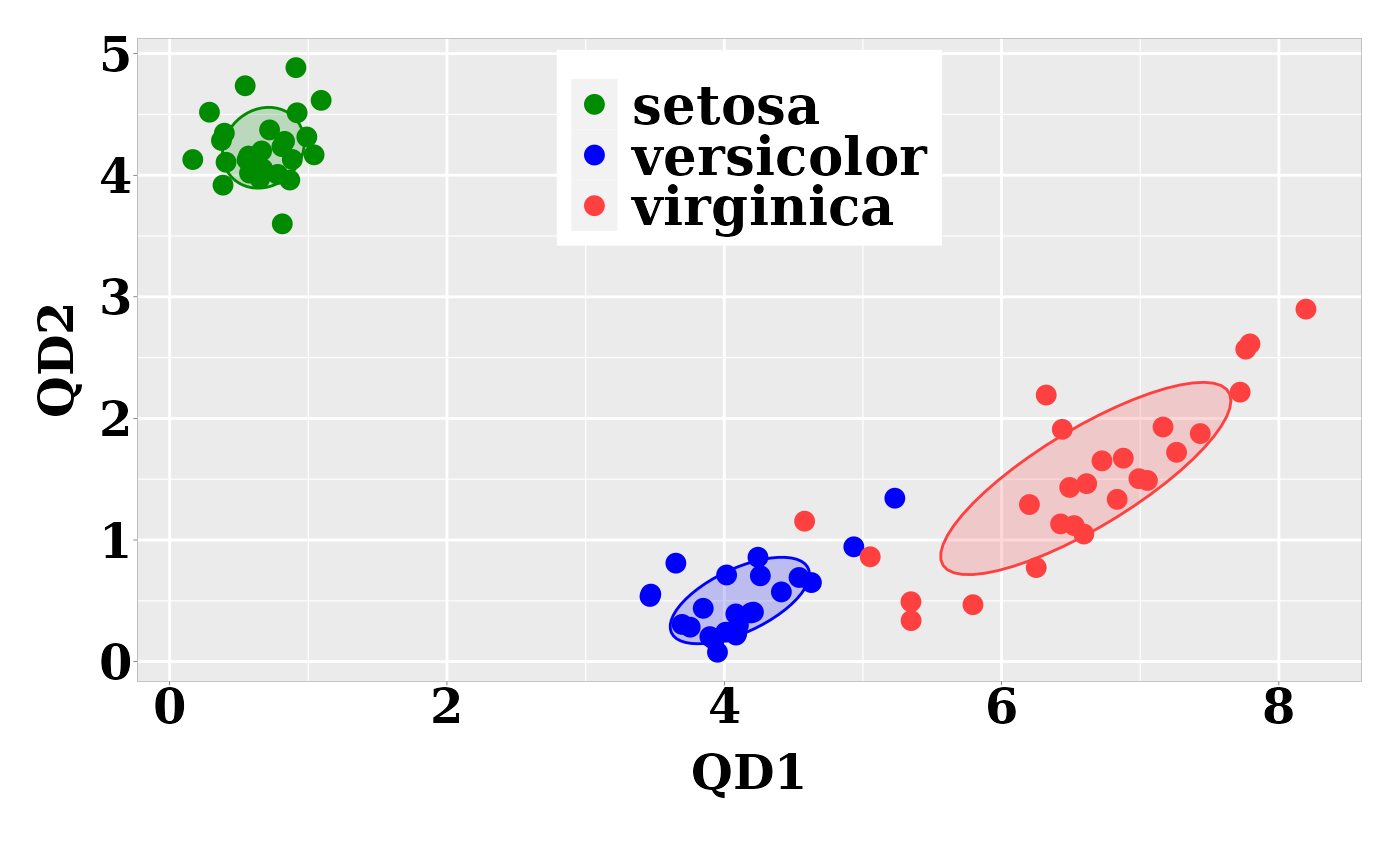
## Graph of the individual quadratic-discriminant scores
require("ggplot2")
dt <- predict(model, newdata = test, type = "qd")
p0 <- theme(
axis.text.x = element_text( face = "bold", size = 18, color="black",
# hjust = 0.5, vjust = 0.5,
family = "serif", angle = 0,
margin = margin(1,0,1,0, unit = "pt" )),
axis.text.y = element_text( face = "bold", size = 18, color="black",
family = "serif",
margin = margin( 0,0.1,0,0, unit = "mm" )),
axis.title.x = element_text(face = "bold", family = "serif", size = 18,
color="black", vjust = 0 ),
axis.title.y = element_text(face = "bold", family = "serif", size = 18,
color="black",
margin = margin( 0,2,0,0, unit = "mm" ) ),
legend.title=element_blank(),
legend.text = element_text(size = 20, face = "bold", family = "serif"),
legend.position = c(0.5, 0.83),
panel.border = element_rect(fill=NA, colour = "black", linewidth=0.07),
panel.grid.minor = element_line(color= "white", linewidth = 0.2),
axis.ticks = element_line(linewidth = 0.1),
axis.ticks.length = unit(0.5, "mm"),
plot.margin = unit(c(1,1,2,1), "lines"))
ggplot(dt, aes(x = QD1, y = QD2, colour = class)) +
geom_point(size = 3) +
scale_color_manual(values = c("green4","blue","brown1")) +
stat_ellipse(aes(x = QD1, y = QD2, fill = class), data = dt,
type = "norm", geom = "polygon", level = 0.5,
alpha=0.2, show.legend = FALSE) +
scale_fill_manual(values = c("green4","blue","brown1")) + p0