Get started-with Methyl-IT
Robersy Sanchez
Department of Biology. Pennsylvania State University, University Park, PA 16802rus547@psu.edu
15 January 2024
Source:vignettes/MethylIT.Rmd
MethylIT.RmdAbstract
A fast introduction into methylation analysis with Methyl-IT is provided here. The methylome analysis implemented in Methyl-IT based on a signal-detection and machine-learning approach. Vignettes with further examples are available at https://genomaths.github.io/methylit/.
Background
MethylIT is an R package for methylome analysis based on a signal-detection machine learning approach (SD-ML). This approach is postulated to provide greater sensitivity for resolving true signal from the methylation background within the methylome (Sanchez and Mackenzie 2016; Sanchez et al. 2019; Sanchez and Mackenzie 2023). Because the biological signal created within the dynamic methylome environment characteristic of plants is not free from background noise, the approach, designated Methyl-IT, includes the application of signal detection theory (Greiner, Pfeiffer, and Smith 2000; Carter et al. 2016; Harpaz et al. 2013; Kruspe et al. 2017). A basic requirement for the application of signal detection is the knowledge of the probability distribution of the background noise, which is used as null hypothesis in the detection of the methylation signal. This probability distribution is, in general, a member of generalized gamma distribution family, and it can be deduced on a statistical mechanical/thermodynamics basis from DNA methylation induced by thermal fluctuations (Sanchez and Mackenzie 2023).
Data sets
Methyl-IT uses the read counts of methylation called derived from whole-genome bisulfite sequencing (WGBS). Methylome datasets of WGBS are available at Gene Expression Omnibus (GEO DataSets). For the current example, we just load RData files containing the read-counts from several samples. Please, notice that we are using here just a toy data set, which permits us to move us fast on Methyl-IT pipeline.
## ===== Download methylation data from PSU's GitLab ========
url <- paste0("https://git.psu.edu/genomath/MethylIT_examples",
            "/raw/master/MethylIT_testing/",
            "memoryLine_100k_samples_cg.RData")
temp <- tempfile(fileext = ".RData")
download.file(url = url, destfile = temp)
load(temp)
file.remove(temp); rm(temp, url)
#> [1] TRUE

names(meth_samples)
#>  [1] "W_3_1" "W_3_2" "W_3_3" "W_3_4" "W_3_5" "M_3_1" "M_3_2" "M_3_3" "M_3_4"
#> [10] "M_3_5"
Gene annotation
Download Arabidopsis thaliana TAIR10 gene annotation data
url <- paste0("https://git.psu.edu/genomath/MethylIT_examples",
            "/raw/master/MethylIT_testing/",
            "Arabidopsis_thaliana.TAIR10.38_only_genes.RData")
temp <- tempfile(fileext = ".RData")
download.file(url = url, destfile = temp)
load(temp)
file.remove(temp); rm(temp, url)
#> [1] TRUE
The reference sample
To perform the comparison between the uncertainty of methylation levels from each group of individuals, control \((c)\) and treatment \((t)\), we should estimate the uncertainty variation with respect to the same reference individual on the mentioned metric space. The reason to measure the uncertainty variation with respect to the same reference resides in that even sibling individuals follow an independent ontogenetic development and, consequently, their developments follow independent stochastic processes. The reference individual is estimated with function poolFromGRlist:
The centroid (of methylation levels) of the group control is used as reference samples. Notice that poolFromGRlist function only uses numerical data. Hence, we must specify the columns carrying the read-count data.
idx <- grep("W", names(meth_samples))
ref <- poolFromGRlist(LR = meth_samples[idx], stat = "mean")
#> *** Building a unique GRanges object from the list...
#>  *** Building coordinates for the new GRanges object ...
#>  *** Strand information is preserved ...
#>
  |
  |                                                                      |   0%
  |
  |==============                                                        |  20%
  |
  |============================                                          |  40%
  |
  |==========================================                            |  60%
  |
  |========================================================              |  80%
  |
  |======================================================================| 100%
#>  *** Sorting by chromosomes and start positions...
#> *** Building a virtual methylome...
Estimation of information divergences
To perform the comparison between the uncertainty of methylation levels from each group of individuals, control \((c)\) and treatment \((t)\), the divergence between the methylation levels of each individual is estimated with respect to the reference sample. This is the step with the highest consumption of computing time.
date()
#> [1] "Mon Jan 15 13:30:35 2024"
ptm <- proc.time()
ml_samples <- meth_samples[c("W_3_1","W_3_2","W_3_3","W_3_4","W_3_5",
                             "M_3_1","M_3_2","M_3_3","M_3_4","M_3_5")]
ml_hd <- estimateDivergence(ref = ref,
                            indiv = ml_samples,
                            Bayesian = TRUE,
                            min.coverage = c(4,4),
                            and.min.cov = FALSE,
                            min.meth = 1,
                            high.coverage = 500,
                            percentile = 0.999,
                            verbose = FALSE)
(proc.time() - ptm)[3]/60 # in min
#>   elapsed
#> 0.1250333
date()
#> [1] "Mon Jan 15 13:30:43 2024"
ml_hd$M_3_1
#> GRanges object with 17782 ranges and 9 metadata columns:
#>           seqnames    ranges strand |        c1        t1        c2        t2
#>              <Rle> <IRanges>  <Rle> | <numeric> <numeric> <numeric> <numeric>
#>       [1]        1       109      + |         3         0         4         0
#>       [2]        1       115      + |         3         0         4         0
#>       [3]        1       161      + |         4         2         5         1
#>       [4]        1       310      + |         6         6         4        12
#>       [5]        1       311      - |         1         3         3         2
#>       ...      ...       ...    ... .       ...       ...       ...       ...
#>   [17778]       Pt     84348      - |         1       210         2       186
#>   [17779]       Pt     84350      + |         2       159         0       133
#>   [17780]       Pt     84351      - |         1       202         2       175
#>   [17781]       Pt     84353      + |         1       153         0       127
#>   [17782]       Pt     84354      - |         1       194         0       164
#>                   p1         p2          TV      bay.TV       hdiv
#>            <numeric>  <numeric>   <numeric>   <numeric>  <numeric>
#>       [1]   0.855530   0.626396    0.000000  -0.2291345 0.31665411
#>       [2]   0.855530   0.626396    0.000000  -0.2291345 0.31665411
#>       [3]   0.628985   0.598198    0.166667  -0.0307872 0.00699817
#>       [4]   0.491634   0.230045   -0.250000  -0.2615884 1.12163729
#>       [5]   0.274564   0.422201    0.350000   0.1476369 0.13205713
#>       ...        ...        ...         ...         ...        ...
#>   [17778] 0.00636821 0.01237291  0.00589896  0.00600470   0.199262
#>   [17779] 0.01451081 0.00266827 -0.01242236 -0.01184254   0.699579
#>   [17780] 0.00661804 0.01312918  0.00637333  0.00651113   0.211982
#>   [17781] 0.00871135 0.00279145 -0.00649351 -0.00591989   0.231223
#>   [17782] 0.00688828 0.00217286 -0.00512821 -0.00471543   0.238154
#>   -------
#>   seqinfo: 7 sequences from an unspecified genome; no seqlengths
Function estimateDivergence returns a list of GRanges objects with the four columns of counts, the information divergence, and additional columns:
- The original matrix of methylated (\(c_i\)) and unmethylated (\(t_i\)) read counts from control (\(i=1\)) and treatment (\(i=2\)) samples.
- “p1” and “p2”: methylation levels for control and treatment, respectively.
- “bay.TV”: total variation \(TV = p_2 - p_1\).
- “TV”: total variation based on simple counts: \(TV=c_1/(c_1+t_1)-c_2/(c_2+t_2)\).
- “hdiv”: Hellinger divergence.
Observe that the absolute values \(|TV|\) is an information divergence as well, which is known as total variation distance (widely used in information theory).
Descriptive statistical analysis
A descriptive analysis on the distribution of Hellinger divergences of methylation levels is recommended. After the raw data filtering introduced with estimateDivergence function, some coverage issue could be detected. Notice that Methyl-IT pipeline assumes that the data quality is good enough.
Like in any other statistical analysis, descriptive statistical analysis help us to detect potential issues in the raw data. It is the user responsibility to perform quality check of his/her dataset before start to apply Methyl-IT. Nevertheless, the quality checking of the raw data is not perfect. So, it is healthy to sees for potential issues.
This is an optional step not included in Methyl-IT. It is up to the user to verify the data quality.
## Critical values
critical.val <- do.call(rbind, lapply(ml_hd, function(x) {
    hd.95 = quantile(x$hdiv, 0.95)
    tv.95 = quantile(abs(x$bay.TV), 0.95)
    btv.95 = quantile(abs(x$TV), 0.95)
    return(c(tv = tv.95, hd = hd.95, bay.TV = btv.95)
    )})
)
critical.val
#>          tv.95%   hd.95% bay.TV.95%
#> W_3_1 0.3119338 1.003136  0.2410714
#> W_3_2 0.3359854 1.100139  0.2500000
#> W_3_3 0.2881010 1.005780  0.2142857
#> W_3_4 0.3177533 1.041646  0.2380952
#> W_3_5 0.2813523 1.075218  0.2090909
#> M_3_1 0.3806664 1.605878  0.3201389
#> M_3_2 0.3711565 1.649375  0.3000000
#> M_3_3 0.4058102 1.734889  0.3333333
#> M_3_4 0.2175861 1.446732  0.2803030
#> M_3_5 0.2281000 1.120914  0.2976190
Quality checking of the coverage
After the raw data filtering introduced with estimateDivergence function, some coverage issue could be detected.
covr <- lapply(ml_hd, function(x) {
                cov <- x$c2 + x$t2
                return(cov)
})

do.call(rbind, lapply(covr, function(x) {
    q60 <- quantile(x, 0.6)
    q9999 <- quantile(x, 0.9999)
    idx1 <- which(x >= q60)
    idx2 <- which(x <= 500)
    q95 <- quantile(x, 0.95)
    idx <- intersect(idx1, idx2)
    return(c(
        round(summary(x)),
        q60, quantile(x, c(0.95, 0.99, 0.999, 0.9999)),
        num.siteGreater_8 = sum(x >= 8),
        q60_to_500 = sum((x >= q60) & (x <= 500)),
        num.siteGreater_500 = sum(x > 500)
))})
)
#>       Min. 1st Qu. Median Mean 3rd Qu. Max. 60%     95%     99%    99.9%
#> W_3_1    0       8     20  273     494 3933  52 1203.00 2028.40 3630.120
#> W_3_2    0       7     21  330     690 2995  53 1450.75 1983.00 2662.000
#> W_3_3    0       8     22  247     434 4013  52 1059.10 1880.84 3661.840
#> W_3_4    0       7     20  293     603 3630  53 1240.30 1891.52 3261.898
#> W_3_5    0       9     21  257     407 4010  52 1149.00 2112.34 3772.608
#> M_3_1    0       7     18  291     580 3421  49 1259.95 1857.57 3131.095
#> M_3_2    0       8     18  253     421 3843  38 1155.00 2006.47 3641.188
#> M_3_3    0       7     16  284     669 2749  36 1193.00 1597.51 2401.004
#> M_3_4    0       8     19  231     399 3975  39  997.00 1968.61 3681.184
#> M_3_5    0       7     16  354     838 3398  38 1494.00 1989.78 3039.694
#>         99.99% num.siteGreater_8 q60_to_500 num.siteGreater_500
#> W_3_1 3890.672             13546       2713                4414
#> W_3_2 2879.331             12904       2392                4705
#> W_3_3 3944.623             13932       3131                4006
#> W_3_4 3550.063             13386       2520                4675
#> W_3_5 3990.634             14631       3254                4098
#> M_3_1 3378.882             13163       2475                4653
#> M_3_2 3799.164             13577       3241                4014
#> M_3_3 2688.904             12393       2492                4687
#> M_3_4 3935.676             13936       3449                3757
#> M_3_5 3323.190             13105       2494                4771
Estimation of the best fitted probability distribution model
A basic requirement for the application of signal detection is the knowledge of the probability distribution of the background noise. Probability distribution, as a Weibull distribution model, can be deduced on a statistical mechanical/thermodynamics basis for DNA methylation induced by thermal fluctuations (Sanchez and Mackenzie 2016).
gof <- gofReport(HD = ml_hd,
                model = c("Weibull2P", "Weibull3P",
                        "Gamma2P", "Gamma3P"),
                column = 9,
                output = "all",
                alt_models = TRUE,
                num.cores = 4L,
                task = 2L,
                verbose = FALSE
)
#>
  |
  |                                                                      |   0%
  |
  |==================                                                    |  25%
  |
  |===================================                                   |  50%
  |
  |====================================================                  |  75%
  |
  |======================================================================| 100%
#>
#>  *** Creating report ...
gof$stats
#>          w2p_AIC w2p_R.Cross.val w3p_AIC w3p_R.Cross.val   g2p_AIC
#> W_3_1  -92604.45       0.9983322     Inf               0 -107319.5
#> W_3_2  -94347.14       0.9985964     Inf               0 -109885.9
#> W_3_3  -96466.50       0.9986544     Inf               0 -114703.9
#> W_3_4  -96546.57       0.9986205     Inf               0 -114453.7
#> W_3_5  -97966.02       0.9985584     Inf               0 -109813.8
#> M_3_1 -106137.75       0.9992454     Inf               0 -127842.1
#> M_3_2 -108524.59       0.9993022     Inf               0 -132209.9
#> M_3_3 -107446.61       0.9993010     Inf               0 -132105.6
#> M_3_4 -124063.33       0.9997121     Inf               0 -119186.2
#> M_3_5 -114904.63       0.9994728     Inf               0 -129744.3
#>       g2p_R.Cross.val g3p_AIC g3p_R.Cross.val bestModel
#> W_3_1       0.9992292     Inf               0       g2p
#> W_3_2       0.9993784     Inf               0       g2p
#> W_3_3       0.9995170     Inf               0       g2p
#> W_3_4       0.9994412     Inf               0       g2p
#> W_3_5       0.9991953     Inf               0       g2p
#> M_3_1       0.9997532     Inf               0       g2p
#> M_3_2       0.9997937     Inf               0       g2p
#> M_3_3       0.9998019     Inf               0       g2p
#> M_3_4       0.9995424     Inf               0       w2p
#> M_3_5       0.9997344     Inf               0       g2p
gof$bestModel
#>       W_3_1       W_3_2       W_3_3       W_3_4       W_3_5       M_3_1
#>   "Gamma2P"   "Gamma2P"   "Gamma2P"   "Gamma2P"   "Gamma2P"   "Gamma2P"
#>       M_3_2       M_3_3       M_3_4       M_3_5
#>   "Gamma2P"   "Gamma2P" "Weibull2P"   "Gamma2P"
Histogram and probability density distribution plot
par(mfcol = c(2,2))
WT1 = ml_hd$W_3_1$hdiv
pars = coef(gof$nlms$W_3_1)
hist(WT1, 90, freq = FALSE, las = 1, family = "serif",
     panel.first={points(0, 0, pch=16, cex=1e6, col="grey95")
       grid(col="white", lty = 1)}, family = "serif", col = "cyan1",
     border = "deepskyblue", xlim = c(0, 2))
x1 <- seq(0, 2, by = 0.001)
lines(x1, dgamma(x1, shape = pars[1], scale = pars[2]), col = "red")

WT2 = ml_hd$W_3_2$hdiv
pars = coef(gof$nlms$W_3_2)
hist(WT2, 90, freq = FALSE, las = 1, family = "serif",
     panel.first={points(0, 0, pch=16, cex=1e6, col="grey95")
       grid(col="white", lty = 1)}, family = "serif", col = "cyan1",
     border = "deepskyblue", xlim = c(0, 2))
x1 <- seq(0, 2, by = 0.001)
lines(x1, dgamma(x1, shape = pars[1], scale = pars[2]), col = "red")

M1 = ml_hd$M_3_1$hdiv
pars = coef(gof$nlms$M_3_1)
hist(M1, 90, freq = FALSE, las = 1, family = "serif",
     panel.first={points(0, 0, pch=16, cex=1e6, col="grey95")
       grid(col="white", lty = 1)}, family = "serif", col = "cyan1",
     border = "deepskyblue", xlim = c(0, 4))
x1 <- seq(0, 4.5, by = 0.001)
lines(x1, dgamma(x1, shape = pars[1], scale = pars[2]), col = "red")

M2 = ml_hd$M_3_2$hdiv
pars = coef(gof$nlms$M_3_2)
hist(M2, 90, freq = FALSE, las = 1, family = "serif",
     panel.first={points(0, 0, pch=16, cex=1e6, col="grey95")
       grid(col="white", lty = 1)}, family = "serif", col = "cyan1",
     border = "deepskyblue", xlim = c(0, 4))
x1 <- seq(0, 4, by = 0.001)
lines(x1, dgamma(x1, shape = pars[1], scale = pars[2]), col = "red")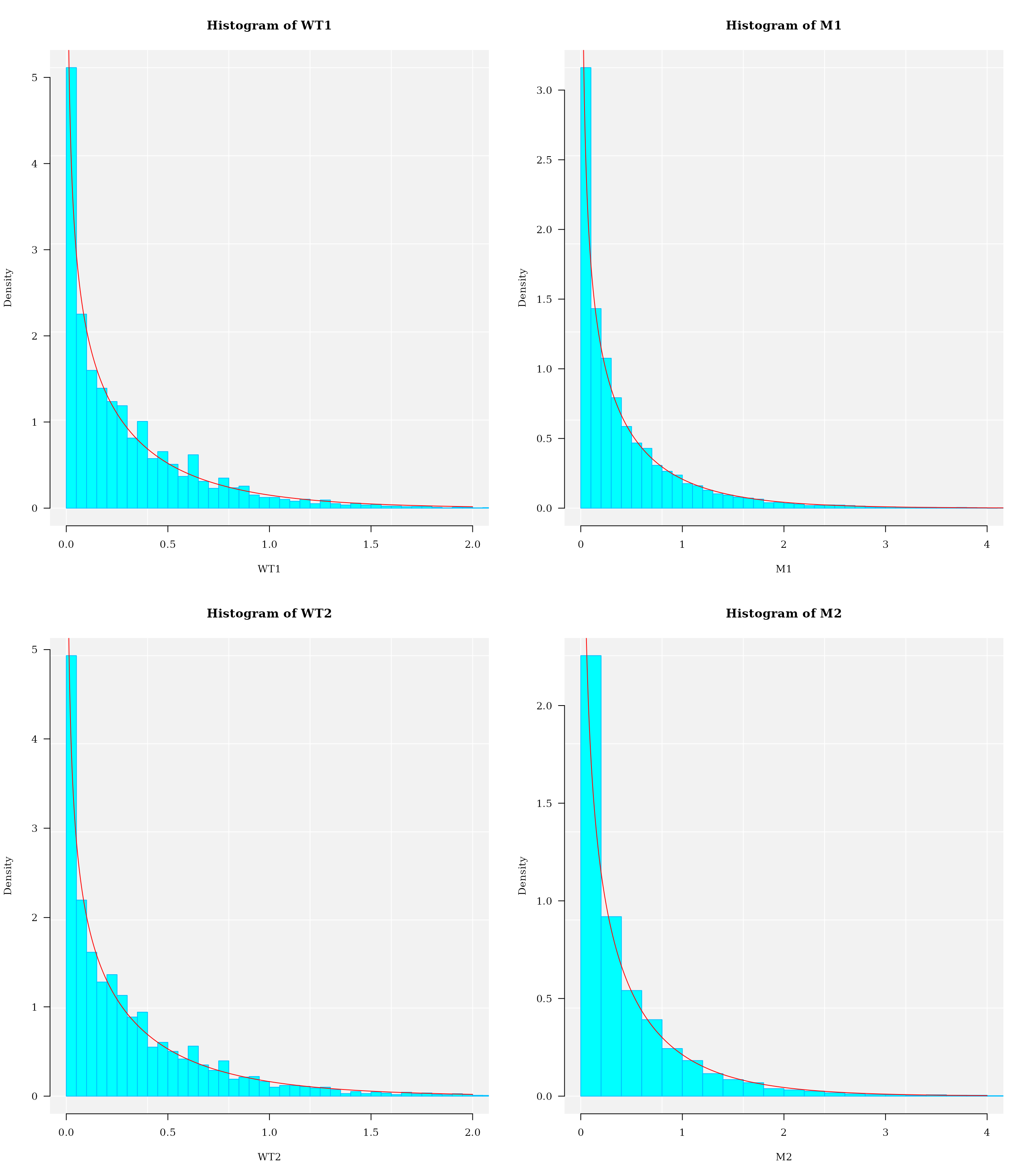
Signal detection
The information thermodynamics-based approach is postulated to provide greater sensitivity for resolving true signal from the thermodynamic background within the methylome (Sanchez and Mackenzie 2016). Since the biological signal created within the dynamic methylome environment characteristic of living organisms is not free from background noise, the approach, designated Methyl-IT, includes the application of signal detection theory (Greiner, Pfeiffer, and Smith 2000; Carter et al. 2016; Harpaz et al. 2013; Kruspe et al. 2017). Signal detection is a critical step to increase sensitivity and resolution of methylation signal by reducing the signal-to-noise ratio and objectively controlling the false positive rate and prediction accuracy/risk.
Potential methylation signal
The first estimation in our signal detection step is the identification of the cytosine sites carrying potential methylation signal \(PS\). The methylation regulatory signal does not hold the theoretical distribution and, consequently, for a given level of significance \(\alpha\) (Type I error probability, e.g. \(\alpha = 0.05\)), cytosine positions \(k\) with information divergence \(H_k >= H_{\alpha = 0.05}\) can be selected as sites carrying potential signals \(PS\). The value of \(\alpha\) can be specified. For example, potential signals with \(H_k > H_{\alpha = 0.01}\) can be selected. For each sample, cytosine sites are selected based on the corresponding fitted theoretical distribution model estimated in the previous step.
ps <- getPotentialDIMP(LR = ml_hd,
                        nlms = gof$nlms,
                        div.col = 9L,
                        tv.col = 8L,
                        tv.cut = 0.25,
                        dist.name = gof$bestModel)
ps$M_3_1
#> GRanges object with 558 ranges and 10 metadata columns:
#>         seqnames    ranges strand |        c1        t1        c2        t2
#>            <Rle> <IRanges>  <Rle> | <numeric> <numeric> <numeric> <numeric>
#>     [1]        1       511      + |        10         5         4         8
#>     [2]        1      5459      + |         6         2         2         5
#>     [3]        1     17641      - |         5         1         1         2
#>     [4]        1     18106      - |         9         0         2         1
#>     [5]        1     24196      + |         6        14        16         0
#>     ...      ...       ...    ... .       ...       ...       ...       ...
#>   [554]        5     93916      - |         0         6         5         3
#>   [555]        5     94024      + |         0        10         3         2
#>   [556]        5     94054      + |         7         2         0         4
#>   [557]        5     94055      - |         5         1         1         5
#>   [558]        5     94058      - |         6         0         4         2
#>                p1        p2        TV    bay.TV      hdiv       wprob
#>         <numeric> <numeric> <numeric> <numeric> <numeric>   <numeric>
#>     [1]  0.650294  0.291535 -0.333333 -0.358759   1.91758 3.24985e-02
#>     [2]  0.712218  0.237111 -0.464286 -0.475107   2.04140 2.70927e-02
#>     [3]  0.773595  0.228468 -0.500000 -0.545127   1.64587 4.86429e-02
#>     [4]  0.942954  0.396115 -0.333333 -0.546839   2.32267 1.79839e-02
#>     [5]  0.303585  0.862793  0.700000  0.559208   6.73007 3.88975e-05
#>     ...       ...       ...       ...       ...       ...         ...
#>   [554] 0.0505441 0.4890867  0.625000  0.438543   2.30405  0.01847590
#>   [555] 0.0320215 0.4222008  0.600000  0.390179   2.10990  0.02450879
#>   [556] 0.7412423 0.0520884 -0.777778 -0.689154   4.10998  0.00142952
#>   [557] 0.7735955 0.1520139 -0.666667 -0.621582   3.06476  0.00620988
#>   [558] 0.9182058 0.4866520 -0.333333 -0.431554   1.77271  0.04026507
#>   -------
#>   seqinfo: 7 sequences from an unspecified genome; no seqlengths
Cutpoint estimation. DMPs
Laws of statistical physics can account for background methylation, a response to thermal fluctuations that presumably functions in DNA stability (Sanchez and Mackenzie 2016; Sanchez et al. 2019). True signal is detected based on the optimal cutpoint (López-Ratón et al. 2014).
The need for the application of (what is now known as) signal detection in cancer research was pointed out by Youden in the midst of the last century (Youden 1950). In the next example, the simple cutpoint estimation available in Methyl-IT is based on the application of Youden index (Youden 1950). Although cutpoints are estimated for a single variable, the classification performance can be evaluated for several variables and applying different model classifiers. A optimal cutpoint distinguishes disease stages from healthy individual. The performance of this classification is given in the output of function estimateCutPoint.
A model classifier can be requested for further predictions and its classification performance is also provided. Below, the selected model classifier is a quadratic discriminant analysis (QDA) (classifier1 = “qda”, clas.perf = TRUE). Four predictor variables are available: the Hellinger divergence of methylation levels (hdiv), total variation distance (TV, absolute difference of methylation levels), relative position of cytosine site in the chromosome (pos), and the logarithm base two of the probability to observe a Hellinger divergence value \(H\) greater than the critical value \(H_{\alpha = 0.05}\) (values given as probabilities in object PS, wprob).
Notice that the cutpoint can be estimated for any of the two currently available information divergences: Hellinger divergence (div.col = 9) or the total variation distance (with Bayesian correction, div.col = 8).
### Cutpoint estimated using a model classifier
cutpoint <- estimateCutPoint(LR = ps,
                            simple = FALSE,
                            div.col = 9,
                            control.names = c("W_3_1","W_3_2","W_3_3",
                                              "W_3_4","W_3_5"),
                            treatment.names = c("M_3_1","M_3_2","M_3_3",
                                                "M_3_4","M_3_5"),
                            column = c(hdiv = TRUE, bay.TV = TRUE,
                                        wprob = TRUE, pos = TRUE),
                            classifier1 = "logistic", n.pc = 4,
                            classifier2 = "pca.qda",
                            center = TRUE,
                            scale = TRUE,
                            clas.perf = TRUE,
                            verbose = FALSE
)
cutpoint$cutpoint
#> [1] 1.018108
cutpoint$testSetPerformance
#> Confusion Matrix and Statistics
#>
#>           Reference
#> Prediction  CT  TT
#>         CT 391   0
#>         TT  22 696
#>
#>                Accuracy : 0.9802
#>                  95% CI : (0.9701, 0.9875)
#>     No Information Rate : 0.6276
#>     P-Value [Acc > NIR] : < 2.2e-16
#>
#>                   Kappa : 0.9571
#>
#>  Mcnemar's Test P-Value : 7.562e-06
#>
#>             Sensitivity : 1.0000
#>             Specificity : 0.9467
#>          Pos Pred Value : 0.9694
#>          Neg Pred Value : 1.0000
#>              Prevalence : 0.6276
#>          Detection Rate : 0.6276
#>    Detection Prevalence : 0.6474
#>       Balanced Accuracy : 0.9734
#>
#>        'Positive' Class : TT
#>
cutpoint$testSetModel.FDR
#> [1] 0
Differentially methylated positions (DMPs) can be now identified using selectDIMP function
dmps <- selectDIMP(ps, div.col = 9, cutpoint = cutpoint$cutpoint)
data.frame(dmps =unlist(lapply(dmps, length)))
#>       dmps
#> W_3_1  354
#> W_3_2  342
#> W_3_3  303
#> W_3_4  383
#> W_3_5  277
#> M_3_1  558
#> M_3_2  450
#> M_3_3  471
#> M_3_4  161
#> M_3_5  252
Differentially methylated genes (DMGs)
Differentially methylated genes (DMGs) are estimated from group comparisons for the number of DMPs on gene-body regions between control and treatment.
Function getDIMPatGenes is used to count the number of DMPs at gene-body. Nevertheless, it can be used for any arbitrary specified genomic region as well. The operation of this function is based on the ‘findOverlaps’ function from the ‘GenomicRanges’ Bioconductor R package. The ‘findOverlaps’ function has several critical parameters like, for example, ‘maxgap’, ‘minoverlap’, and ‘ignore.strand’. In our function getDIMPatGenes, except for setting ignore.strand = TRUE and type = “within”, we preserve the rest of default ‘findOverlaps’ parameters. In this case, these are important parameter settings because the local mechanical effect of methylation changes on a DNA region where a gene is located is independent of the strand where the gene is encoded. That is, methylation changes located in any of the two DNA strands inside the gene-body region will affect the flexibility of the DNA molecule (Choy et al. 2010; Severin et al. 2011).
nams <- names(dmps)
dmps_at_genes <- getDIMPatGenes(GR = dmps, GENES = genes, ignore.strand = TRUE)
dmps_at_genes <- uniqueGRanges(dmps_at_genes, columns = 2L,
                                ignore.strand = TRUE, type = "equal",
                               verbose = FALSE)
colnames(mcols(dmps_at_genes)) <- nams
dmps_at_genes
#> GRanges object with 70 ranges and 10 metadata columns:
#>        seqnames      ranges strand |     W_3_1     W_3_2     W_3_3     W_3_4
#>           <Rle>   <IRanges>  <Rle> | <numeric> <numeric> <numeric> <numeric>
#>    [1]        1   3631-5899      * |         0         0         0         1
#>    [2]        1   6788-9130      * |         0         0         0         0
#>    [3]        1 23121-31227      * |        12         8        17         5
#>    [4]        1 31170-33171      * |         2         0         2         0
#>    [5]        1 33365-37871      * |         2         0         1         1
#>    ...      ...         ...    ... .       ...       ...       ...       ...
#>   [66]        5 49891-51437      * |         0         0         1         0
#>   [67]        5 53856-56052      * |         1         0         9         3
#>   [68]        5 61017-63936      * |         2         0         1         0
#>   [69]        5 84474-86275      * |         0         0         0         0
#>   [70]        5 91838-95701      * |         4         1         2         1
#>            W_3_5     M_3_1     M_3_2     M_3_3     M_3_4     M_3_5
#>        <numeric> <numeric> <numeric> <numeric> <numeric> <numeric>
#>    [1]         0         1         2         1         2         1
#>    [2]         0         0         0         1         0         1
#>    [3]         9        11        14        16         9         8
#>    [4]         2         1         0         0         0         0
#>    [5]         1         2         0         1         0         0
#>    ...       ...       ...       ...       ...       ...       ...
#>   [66]         0         2         2         2         2         2
#>   [67]         1         7         4         4         0         1
#>   [68]         1         6         7         2         3         4
#>   [69]         0         0         0         0         0         1
#>   [70]         1         8         2         4         5         4
#>   -------
#>   seqinfo: 5 sequences from an unspecified genome; no seqlengths
Setting the experiment design
The experimental design is set with glmDataSet function
colData <- data.frame(condition = factor(c("WT", "WT", "WT", "WT", "WT",
                                            "ML", "ML", "ML", "ML", "ML"),
                                        levels = c("WT", "ML")),
                    nams,
                    row.names = 2)
## A RangedGlmDataSet is created
ds <- glmDataSet(GR = dmps_at_genes, colData = colData)
Testing for DMGs
DMGs are detected using function countTest2.
dmgs <- countTest2(DS = ds, num.cores = 4L,
                    tasks = 2L,
                    minCountPerIndv = 7,
                    CountPerBp = 0.001,
                    test = "LRT",
                    verbose = TRUE)
#> *** Number of GR after filtering counts 3
#> *** GLM...
dmgs
#> GRanges object with 1 range and 18 metadata columns:
#>       seqnames      ranges strand |     W_3_1     W_3_2     W_3_3     W_3_4
#>          <Rle>   <IRanges>  <Rle> | <numeric> <numeric> <numeric> <numeric>
#>   [1]        3 31145-34670      * |         3         2         3         4
#>           W_3_5     M_3_1     M_3_2     M_3_3     M_3_4     M_3_5    log2FC
#>       <numeric> <numeric> <numeric> <numeric> <numeric> <numeric> <numeric>
#>   [1]         3         6         8         9         6         7  0.875469
#>       scaled.deviance      pvalue          model    adj.pval CT.SignalDensity
#>             <numeric>   <numeric>    <character>   <numeric>        <numeric>
#>   [1]         67.8239 1.78768e-16 Neg.Binomial.W 1.78768e-16      0.000850822
#>       TT.SignalDensity SignalDensityVariation
#>              <numeric>              <numeric>
#>   [1]       0.00204197             0.00119115
#>   -------
#>   seqinfo: 1 sequence from an unspecified genome; no seqlengths
References
Session info
Here is the output of sessionInfo() on the system on
which this document was compiled running pandoc 3.1.1:
#> R version 4.3.2 (2023-10-31)
#> Platform: x86_64-pc-linux-gnu (64-bit)
#> Running under: Ubuntu 22.04.3 LTS
#>
#> Matrix products: default
#> BLAS:   /usr/lib/x86_64-linux-gnu/blas/libblas.so.3.10.0
#> LAPACK: /usr/lib/x86_64-linux-gnu/lapack/liblapack.so.3.10.0
#>
#> locale:
#>  [1] LC_CTYPE=en_US.UTF-8       LC_NUMERIC=C
#>  [3] LC_TIME=en_US.UTF-8        LC_COLLATE=en_US.UTF-8
#>  [5] LC_MONETARY=en_US.UTF-8    LC_MESSAGES=en_US.UTF-8
#>  [7] LC_PAPER=en_US.UTF-8       LC_NAME=C
#>  [9] LC_ADDRESS=C               LC_TELEPHONE=C
#> [11] LC_MEASUREMENT=en_US.UTF-8 LC_IDENTIFICATION=C
#>
#> time zone: America/New_York
#> tzcode source: system (glibc)
#>
#> attached base packages:
#> [1] stats4    stats     graphics  grDevices utils     datasets  methods
#> [8] base
#>
#> other attached packages:
#> [1] MethylIT_0.3.2.7     rtracklayer_1.60.1   GenomicRanges_1.52.1
#> [4] GenomeInfoDb_1.36.4  IRanges_2.34.1       S4Vectors_0.38.2
#> [7] BiocGenerics_0.46.0  BiocStyle_2.28.1
#>
#> loaded via a namespace (and not attached):
#>   [1] rstudioapi_0.15.0           jsonlite_1.8.7
#>   [3] magrittr_2.0.3              rmarkdown_2.25
#>   [5] fs_1.6.3                    BiocIO_1.10.0
#>   [7] zlibbioc_1.46.0             ragg_1.2.6
#>   [9] vctrs_0.6.5                 memoise_2.0.1
#>  [11] Rsamtools_2.16.0            RCurl_1.98-1.13
#>  [13] htmltools_0.5.7             S4Arrays_1.0.6
#>  [15] pROC_1.18.5                 caret_6.0-94
#>  [17] sass_0.4.8                  parallelly_1.36.0
#>  [19] bslib_0.6.1                 desc_1.4.3
#>  [21] plyr_1.8.9                  lubridate_1.9.3
#>  [23] cachem_1.0.8                GenomicAlignments_1.36.0
#>  [25] lifecycle_1.0.4             minpack.lm_1.2-4
#>  [27] iterators_1.0.14            pkgconfig_2.0.3
#>  [29] Matrix_1.6-4                R6_2.5.1
#>  [31] fastmap_1.1.1               GenomeInfoDbData_1.2.10
#>  [33] MatrixGenerics_1.12.3       future_1.33.0
#>  [35] digest_0.6.33               colorspace_2.1-0
#>  [37] AnnotationDbi_1.62.2        textshaping_0.3.7
#>  [39] RSQLite_2.3.3               randomForest_4.7-1.1
#>  [41] fansi_1.0.6                 timechange_0.2.0
#>  [43] httr_1.4.7                  abind_1.4-5
#>  [45] compiler_4.3.2              proxy_0.4-27
#>  [47] bit64_4.0.5                 withr_2.5.2
#>  [49] BiocParallel_1.34.2         DBI_1.1.3
#>  [51] highr_0.10                  MASS_7.3-60
#>  [53] lava_1.7.3                  DelayedArray_0.26.7
#>  [55] rjson_0.2.21                ModelMetrics_1.2.2.2
#>  [57] tools_4.3.2                 future.apply_1.11.0
#>  [59] nnet_7.3-19                 glue_1.6.2
#>  [61] restfulr_0.0.15             nlme_3.1-164
#>  [63] grid_4.3.2                  reshape2_1.4.4
#>  [65] generics_0.1.3              recipes_1.0.8
#>  [67] gtable_0.3.4                class_7.3-22
#>  [69] data.table_1.14.8           utf8_1.2.4
#>  [71] XVector_0.40.0              foreach_1.5.2
#>  [73] pillar_1.9.0                stringr_1.5.1
#>  [75] genefilter_1.82.1           splines_4.3.2
#>  [77] dplyr_1.1.4                 lattice_0.22-5
#>  [79] survival_3.5-7              bit_4.0.5
#>  [81] annotate_1.78.0             tidyselect_1.2.0
#>  [83] Biostrings_2.68.1           knitr_1.45
#>  [85] bookdown_0.37               SummarizedExperiment_1.30.2
#>  [87] xfun_0.41                   Biobase_2.60.0
#>  [89] hardhat_1.3.0               timeDate_4022.108
#>  [91] matrixStats_1.2.0           proto_1.0.0
#>  [93] stringi_1.8.3               yaml_2.3.8
#>  [95] evaluate_0.23               codetools_0.2-19
#>  [97] tibble_3.2.1                BiocManager_1.30.22
#>  [99] cli_3.6.2                   nls2_0.3-3
#> [101] rpart_4.1.23                xtable_1.8-4
#> [103] systemfonts_1.0.5           munsell_0.5.0
#> [105] jquerylib_0.1.4             Rcpp_1.0.11
#> [107] globals_0.16.2              png_0.1-8
#> [109] XML_3.99-0.16               parallel_4.3.2
#> [111] pkgdown_2.0.7               gower_1.0.1
#> [113] ggplot2_3.4.4               blob_1.2.4
#> [115] bitops_1.0-7                listenv_0.9.0
#> [117] ipred_0.9-14                e1071_1.7-13
#> [119] scales_1.3.0                prodlim_2023.08.28
#> [121] purrr_1.0.2                 crayon_1.5.2
#> [123] rlang_1.1.2                 KEGGREST_1.40.1