Methylation analysis with Methyl-IT
An example with simulated datasets. A guide for users
An example with simulated datasets. A guide for users
Robersy Sanchez
rus547@psu.edu
Mackenzie’s lab
Department of Biology and Plant Science.
Pennsylvania State University, University Park, PA 16802
rus547@psu.edu
Mackenzie’s lab
Department of Biology and Plant Science.
Pennsylvania State University, University Park, PA 16802
15 January 2024
Source:vignettes/Methylation_analysis_with_Methyl-IT.Rmd
Methylation_analysis_with_Methyl-IT.RmdAbstract
Methylation analysis with Methyl-IT is illustrated on simulated datasets of methylated and unmethylated read counts with relatively high average of methylation levels: 0.15 and 0.286 for control and treatment groups, respectively. The main Methyl-IT downstream analysis is presented alongside the application of Fisher’s exact test. The importance of a signal detection step is shown.
Background
Methyl-IT R package offers a methylome analysis approach based on information thermodynamics (IT) and signal detection. Methyl-IT approach confront detection of differentially methylated cytosine as a signal detection problem. This approach was designed to discriminate methylation regulatory signal from background noise induced by molecular stochastic fluctuations. Methyl-IT R package is not limited to the IT approach but also includes Fisher’s exact test (FT), Root-mean-square statistic (RMST) or Hellinger divergence (HDT) tests. Herein, we will show that a signal detection step is also required for FT, RMST, and HDT as well. It is worthy to notice that, as for any standard statistical analysis, any serious robust methylation analysis requires for a descriptive statistical analysis at the beginning or at different downstream steps. This is an ABC principle taught in any undergraduate course on statistics. Methylation analysis is not the exception of the rule. This detail is included in this example.
Note: This example was made with the MethylIT version at https://github.com/genomaths/MethylIT.
Available datasets and reading
Methylome datasets of whole-genome bisulfite sequencing (WGBS) are available at Gene Expression Omnibus (GEO DataSets). The data set are downloaded providing the GEO accession numbers for each data set to the function getGEOSuppFiles (for details type ?getGEOSuppFiles in the R console). Then, datasets can be read using function readCounts2GRangesList. An example on how to load datasets of read-counts of methylated and unmethylated cytosine into Methyl-IT is given in the Cancer example at https://git.psu.edu/genomath/MethylIT
Data generation
For the current example on methylation analysis with Methyl-IT we will use simulated data. Read-count matrices of methylated and unmethylated cytosine are generated with Methyl-IT function simulateCounts.
Function simulateCounts randomly generates prior methylation levels using Beta distribution function. The expected mean of methylation levels that we would like to have can be estimated using the auxiliary function:
bmean <- function(alpha, beta) alpha/(alpha + beta)
alpha.ct <- 0.09
alpha.tt <- 0.2
c(control.group = bmean(alpha.ct, 0.5), treatment.group = bmean(alpha.tt, 0.5),
    mean.diff = bmean(alpha.tt, 0.5) - bmean(alpha.ct, 0.5))
## control.group treatment.group mean.diff
## 0.1525424 0.2857143 0.1331719This simple function uses the \(\alpha\) (shape1) and \(\beta\) (shape2) parameters from the Beta distribution function to compute the expected value of methylation levels. In the current case, we expect to have a difference of methylation levels about 0.133 between the control and the treatment.
Simulation
Function simulateCounts from MethylIT.utils R package will be used to generate the datasets, which will include three group of samples: reference, control, and treatment.
library(MethylIT)
library(MethylIT.utils)
library(BiocParallel)

# The number of cytosine sites to generate
sites = 50000
# Set a seed for pseudo-random number generation
set.seed(124)
control.nam <- c("C1", "C2", "C3")
treatment.nam <- c("T1", "T2", "T3")

# Reference group
ref0 = simulateCounts(num.samples = 4, sites = sites, alpha = alpha.ct,
                    beta = 0.5, size = 50, theta = 4.5,
                    sample.ids = c("R1", "R2", "R3", "R4"))
# Control group
ctrl = simulateCounts(num.samples = 3, sites = sites, alpha = alpha.ct,
                    beta = 0.5, size = 50, theta = 4.5,
                    sample.ids = control.nam)
# Treatment group
treat = simulateCounts(num.samples = 3, sites = sites, alpha = alpha.tt,
                    beta = 0.5, size = 50, theta = 4.5,
                    sample.ids = treatment.nam)
Notice that reference and control groups of samples are not identical but belong to the same population.
Divergences of methylation levels
The estimation of the divergences of methylation levels is required to proceed with the application of signal detection basic approach. The information divergence is estimated here using the function estimateDivergence. For each cytosine site, methylation levels are estimated according to the formulas: \(p_i={n_i}^{mC_j}/({n_i}^{mC_j}+{n_i}^{C_j})\), where \({n_i}^{mC_j}\) and \({n_i}^{C_j}\) are the number of methylated and unmethylated cytosines at site \(i\).
If a Bayesian correction of counts is selected in function estimateDivergence, then methylated read counts are modeled by a beta-binomial distribution in a Bayesian framework, which accounts for the biological and sampling variations (1–3). In our case we adopted the Bayesian approach suggested in reference (4) (Chapter 3).
Two types of information divergences are estimated: TV, total variation (TV, absolute value of methylation levels) and Hellinger divergence (H). TV is computed according to the formula: \(TV_d=|p_{tt}-p_{ct}|\) and H:
\[H(\hat p_{ij},\hat p_{ir}) = w_i\Big[(\sqrt{\hat p_{ij}} - \sqrt{\hat p_{ir}})^2+(\sqrt{1-\hat p_{ij}} - \sqrt{1-\hat p_{ir}})^2\Big]\] where \(w_i = 2 \frac{m_{ij} m_{ir}}{m_{ij} + m_{ir}}\), \(m_{ij} = {n_i}^{mC_j}+{n_i}^{uC_j}+1\), \(m_{ir} = {n_i}^{mC_r}+{n_i}^{uC_r}+1\) and \(j \in {\{c,t}\}\)
The equation for Hellinger divergence is given in reference (5), but any other information theoretical divergences could be used as well.
Divergences are estimated for control and treatment groups in respect to a virtual sample, which is created applying function poolFromGRlist on the reference group.
# Reference sample
ref = poolFromGRlist(ref0, stat = "mean", num.cores = 4L, verbose = FALSE)

# Methylation level divergences
DIVs <- estimateDivergence(
                        ref = ref,
                        indiv = c(ctrl, treat),
                        Bayesian = TRUE,
                        and.min.cov = FALSE,
                        num.cores = multicoreWorkers(),
                        percentile = 1,
                        verbose = FALSE)
The setting and.min.cov = TRUE in estimateDivergence will accomplish pairwise deletion of missing cytosine sites or sites no holding the filtering condition. The mean of methylation levels differences is:
##           C1           C2           C3           T1           T2           T3
## 2.809709e-03 2.642337e-03 7.127907e-05 1.615112e-01 1.631192e-01 1.642946e-01
Methylation signal
Likewise for any other signal in nature, the analysis of methylation signal requires for the knowledge of its probability distribution. In the current case , the signal is represented in terms of the Hellinger divergence of methylation levels (H).
# To remove hd == 0 to estimate. The methylation signal only is given for
divs = lapply(DIVs, function(div) div[ div$hdiv > 0 ], keep.attr = TRUE)
names(divs) <- names(DIVs)

# Data frame with the Hellinger divergences from both groups of samples samples
l = c(); for (k in 1:length(divs)) l = c(l, length(divs[[k]]))
data_div <- data.frame(H = c(abs(divs$C1$hdiv), abs(divs$C2$hdiv),
                            abs(divs$C3$hdiv), abs(divs$T1$hdiv),
                            abs(divs$T2$hdiv), abs(divs$T3$hdiv)),
                    sample = c(rep("C1", l[1]), rep("C2",l[2]), rep("C3",l[3]),
                                rep("T1",l[4]), rep("T2",l[5]), rep("T3",l[6]))
)
Empirical critical values for the probability distribution of \(H\) and \(TV\) can be obtained using quantile function from the R package stats.
critical.val <- do.call(rbind, lapply(divs, function(x) {
    hd.95 = quantile(x$hdiv, 0.95)
    tv.95 = quantile(abs(x$bay.TV), 0.95)
    return(c(tv = tv.95, hd = hd.95))
}))

critical.val
## tv.95% hd.95%
## C1 0.6732098 66.76003
## C2 0.6707588 66.71971
## C3 0.6669981 65.98486
## T1 0.9232609 138.68200
## T2 0.9318191 141.72617
## T3 0.9301631 141.77236The kernel density estimation yields the empirical density shown in the graphics:
suppressMessages(library(ggplot2))

# Some information for graphic
crit.val.ct <- round(max(critical.val[c("C1", "C2", "C3"), 2])) # 67
crit.val.tt <- round(min(critical.val[c("T1", "T2", "T3"), 2])) # 139

# Density plot with ggplot
ggplot(data_div, aes(x = H, colour = sample, fill = sample)) +
    geom_density(alpha = 0.05, bw = 0.2, position = "identity", na.rm = TRUE,
            linewidth = 0.4) +
    xlab(expression(bolditalic("Hellinger divergence (H)"))) +
    ylab(expression(bolditalic("Density"))) +
    ggtitle("Density distribution for control and treatment") +
    geom_vline(xintercept = crit.val.ct, color = "red",
                linetype = "dashed", linewidth = 0.4) +
    annotate(geom = "text", x = crit.val.ct-2, y = 0.08, size = 5,
            label = 'bolditalic(H[alpha == 0.05]^CT == 67)',
            family = "serif", color = "red", parse = TRUE) +
    geom_vline(xintercept = crit.val.tt, color = "blue",
                linetype = "dashed", linewidth = 0.4) +
    annotate(geom = "text", x = crit.val.tt -2, y = 0.1, size = 5,
            label = 'bolditalic(H[alpha == 0.05]^TT == 139)',
            family = "serif", color = "blue", parse = TRUE) +
    theme(
        axis.text.x  = element_text( face = "bold", size = 12, color="black",
                                margin = margin(1,0,1,0, unit = "pt" )),
        axis.text.y  = element_text( face = "bold", size = 12, color="black",
                                margin = margin( 0,0.1,0,0, unit = "mm")),
        axis.title.x = element_text(face = "bold", size = 13,
                                color="black", vjust = 0 ),
        axis.title.y = element_text(face = "bold", size = 13,
                                color="black", vjust = 0 ),
        legend.title = element_blank(),
        legend.margin = margin(c(0.3, 0.3, 0.3, 0.3), unit = 'mm'),
        legend.box.spacing = unit(0.5, "lines"),
        legend.text = element_text(face = "bold", size = 12, family = "serif")
    )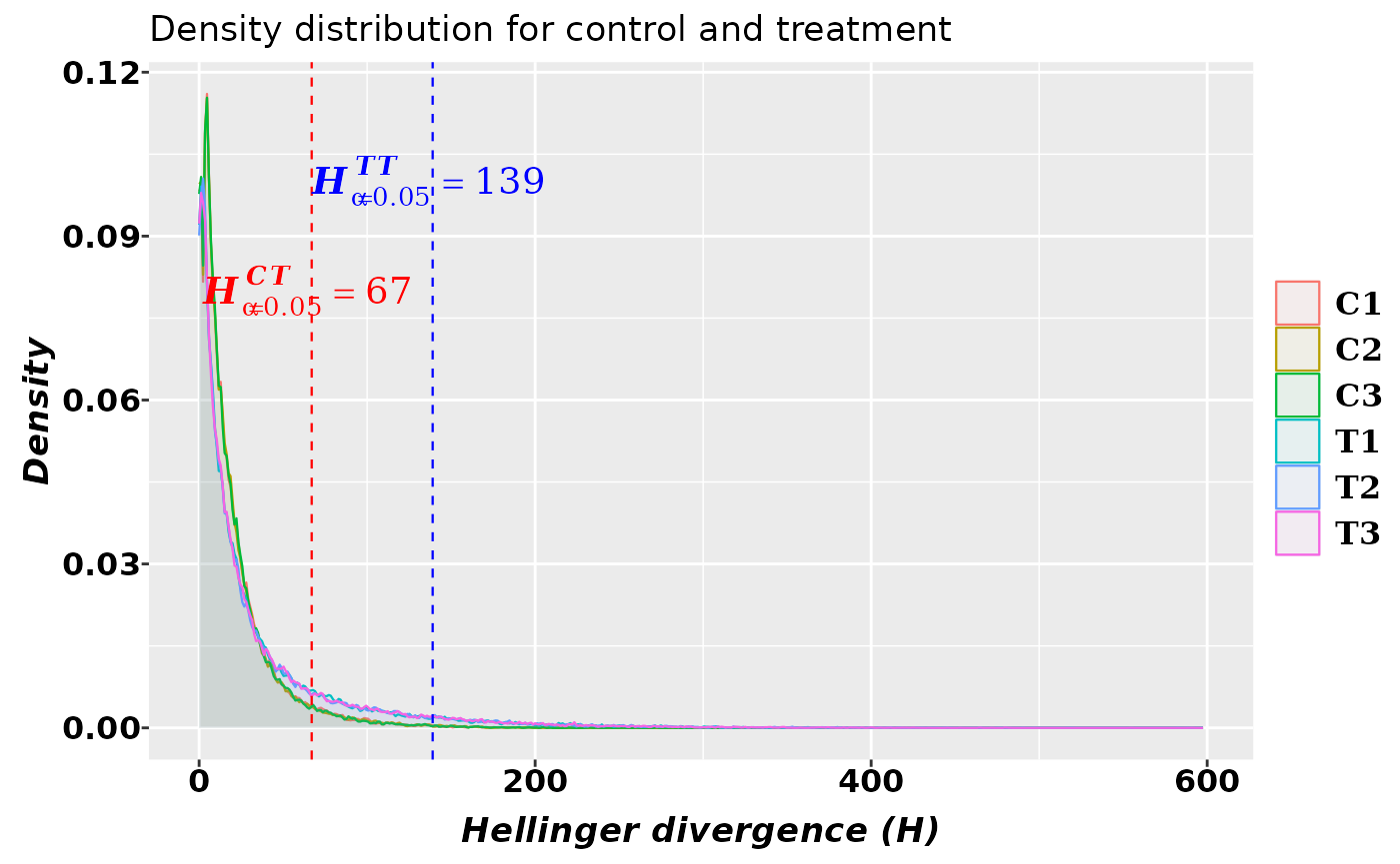
The graphic above shows that with high probability the methylation signal induced by the treatment has H values \(H^{TT}_{\alpha=0.05}\geq139\). According to the critical value estimated for the differences of methylation levels, the methylation signal holds \(TV^{TT}_{\alpha=0.05}\geq0.67\).
Notice that most of the methylation changes are not signal but methylation background noise (found to the left of the critical values). This situation is typical for all the natural and technologically generated signals (6, 7).
Signal detection
Signal detection is a critical step to increase sensitivity and resolution of methylation signal by reducing the signal-to-noise ratio and objectively controlling the false positive rate and prediction accuracy/risk.
The first estimation in our signal detection step is the identification of the cytosine sites carrying potential methylation signal \(PS\). To identify cytosine sites carrying \(PS\), we must find the best fitted probability distribution model.
Estimation of the best fitted probability distribution model
Potential DMPs can be estimated using the critical values derived from the best fitted probability distribution model, which is obtained after the non-linear fit of the theoretical model on the genome-wide \(H\) values for each individual sample using Methyl-IT function nonlinearFitDist (6). As before, only cytosine sites with critical values \(TV_d>0.926\) are considered DMPs. Notice that, it is always possible to use any other values of \(H\) and \(TV_d\) as critical values, but whatever could be the value it will affect the final accuracy of the classification performance of DMPs into two groups, DMPs from control and DMPs from treatment (see below). So, it is important to do an good choices of the critical values.
Function gofReport search for the best fitted model between the set of models requested by the user.
d <- c("Weibull2P", "Weibull3P", "Gamma2P", "Gamma3P", "GGamma3P")
gof <- gofReport(HD = DIVs, column = 9L, model = d, num.cores = 4L,
            tasks = 2L, output = "all", verbose = FALSE)
gof$bestModel
There is not a one-to-one mapping between \(TV_d\) and \(H\). However, at each cytosine site \(i\), these information divergences hold the inequality: \[TV_d(p^{tt}_i,p^{ct}_i)\leq \sqrt{2}H_d(p^{tt}_i,p^{ct}_i)\]
where \(H_d(p^{tt}_i,p^{ct}_i)=\sqrt{\frac{H(p^{tt}_i,p^{ct}_i)}w}\) is the Hellinger distance and \(H(p^{tt}_i,p^{ct}_i)\) is the Hellinger divergence equation given above.
Potential methylation signal
Methylation regulatory signals do not hold the theoretical distribution and, consequently, for a given level of significance \(\alpha\) (Type I error probability, e.g. \(\alpha = 0.05\)), cytosine positions \(k\) with information divergence \(H_k >= H_{\alpha = 0.05}\) can be selected as sites carrying potential signals \(PS\). The \(PS\) is detected with the function getPotentialDIMP.
PS = getPotentialDIMP(LR = DIVs, dist.name = gof$bestModel, nlms = gof$nlms,
                    div.col = 9, alpha = 0.05, tv.col = 8, tv.cut =  0.674)
Observe that we have used the \(|TV|\) values based on the Bayesian estimation of methylation levels (bay.TV, tv.col = 8).
Potential DMPs detected with Fisher’s exact test (FT)
Fisher’s exact test (FT) is run here as standard alternative approach. A full discussion on the performance of FT and other statistical approaches in comparison with Methyl-IT pipeline can be read in (7). Notice that the standard application of FT does not include a signal detection step (see more at (7)).
In Methyl-IT, FT is implemented in function FisherTest. In the current case, a pairwise group application of FT to each cytosine site is performed. The differences between the group means of read counts of methylated and unmethylated cytosines at each site are used for testing (\(pooling.stat ="mean"\)). Notice that only cytosine sites with critical values \(TV_d>0.67\) are tested (tv.cut = 0.67).
ft = FisherTest(LR = divs, tv.cut = 0.67,
                    pAdjustMethod = "BH",  pooling.stat = "mean",
                    pvalCutOff = 0.05, num.cores = multicoreWorkers(),
                    verbose = FALSE, saveAll = FALSE)

# TV column is the standard TV value (without Bayesian correction of methylation
# levels)
ft.tv <- getPotentialDIMP(LR = ft, div.col = 9L, dist.name = "None",
                        tv.cut = 0.67, tv.col = 7, alpha = 0.05)
The above setting would impose additional constrains on the output of DMPs resulting from Fisher’s exact test depending on how strong is the methylation background noise in the control population. Basically, methylation variations that can spontaneously occur in the control population with relatively high frequencies are disregarded. The decisions are based on the empirical cumulative distribution function (ECDF).
Potential DMPs detected with FT can be constrained with the critical values derived for the best fitted probability distribution models
# Potential DMPs from Fisher's exact test
ft.hd <- getPotentialDIMP(LR = ft, div.col = 9L, nlms = gof$nlms,
                        tv.cut = 0.674, tv.col = 8, alpha = 0.05,
                        dist.name = gof$bestModel)
ft.hd$T1
## GRanges object with 2226 ranges and 12 metadata columns:
## seqnames ranges strand | c1 t1 c2 t2
## <Rle> <IRanges> <Rle> | <numeric> <numeric> <numeric> <numeric>
## [1] 1 29 * | 6 110 112 4
## [2] 1 42 * | 0 112 112 0
## [3] 1 70 * | 0 84 84 0
## [4] 1 103 * | 0 94 91 3
## [5] 1 105 * | 0 168 118 50
## ... ... ... ... . ... ... ... ...
## [2222] 1 49928 * | 10 148 158 0
## [2223] 1 49974 * | 19 130 147 2
## [2224] 1 49980 * | 45 139 184 0
## [2225] 1 49981 * | 34 143 177 0
## [2226] 1 49996 * | 20 196 216 0
## p1 p2 TV bay.TV hdiv pvalue
## <numeric> <numeric> <numeric> <numeric> <numeric> <numeric>
## [1] 0.05779995 0.961168 0.913793 0.903368 134.086 1.22001e-52
## [2] 0.00845858 0.995244 1.000000 0.986785 189.744 1.39309e-66
## [3] 0.01112222 0.993674 1.000000 0.982551 138.682 8.69664e-50
## [4] 0.00999781 0.962704 0.968085 0.952706 134.850 1.29337e-50
## [5] 0.00571921 0.700659 0.702381 0.694940 132.207 2.02668e-50
## ... ... ... ... ... ... ...
## [2222] 0.0674516 0.996621 0.936709 0.929170 217.700 1.25471e-78
## [2223] 0.1298691 0.983069 0.859060 0.853200 156.395 3.15691e-60
## [2224] 0.2434358 0.997096 0.755435 0.753661 170.369 1.01280e-61
## [2225] 0.1923356 0.996982 0.807910 0.804647 182.532 2.77686e-66
## [2226] 0.0950087 0.997525 0.907407 0.902516 279.852 2.42409e-100
## adj.pval wprob
## <numeric> <numeric>
## [1] 4.86816e-52 0.0480895
## [2] 1.07813e-65 0.0215268
## [3] 3.03410e-49 0.0448150
## [4] 4.68846e-50 0.0475260
## [5] 7.31951e-50 0.0495093
## ... ... ...
## [2222] 1.67316e-77 0.01487102
## [2223] 1.80286e-59 0.03441153
## [2224] 6.21624e-61 0.02815467
## [2225] 2.11753e-65 0.02375878
## [2226] 9.74758e-99 0.00693179
## -------
## seqinfo: 1 sequence from an unspecified genome; no seqlengthsThe above result shows column ‘adj.pval’ with the FT’s p.values adjusted for multiple comparisons and column ‘wprob’ with the predicted probabilities: \(1 - P(H_k >= H_{\alpha = 0.05})\) from the best fitted model.
Summary table:
data.frame(ft = unlist(lapply(ft.tv, length)),
            ft.hd = unlist(lapply(ft.hd, length)),
BestModel = unlist(lapply(PS, length)))
## ft ft.hd BestModel
## C1 1865 1043 1043
## C2 1824 1075 1075
## C3 1765 1039 1039
## T1 7800 2226 2226
## T2 7847 2167 2167
## T3 7879 2189 2189Notice that there are significant differences between the numbers of PSs detected by FT and other approaches. There at least about 7800 - 2226 = 5574 or more PSs in the treatment samples that are not induced by the treatment, which can naturally occurs in both groups, control and treatment. In other words, the best probabilistic distribution models suggest that those methylation events are resultant of the normal (non-stressful) biological processes. Any information divergence of methylation level below the critical value \(TV_{\alpha=0.05}\) or \(H_{\alpha=0.05}\) is a methylation event that can occur in normal conditions. It does not matter how much significant a test like FT could be, since it is not about the signification of the test, but about how big is the probability to observe that methylation event in the control population as well.
Critical values based on fitted models
Critical values \(H_{\alpha=0.05}\) can be estimated from each fitted model using predict function:
# ==== 95% quantiles
q95 <- data.frame(q95 = predict(object = gof$nlms, pred = "quant", q = 0.95,
                                dist.name = gof$bestModel))
q95
## q95
## C1 59.08915
## C2 58.32001
## C3 58.32643
## T1 131.57161
## T2 137.55786
## T3 136.17154Cutpoint for the spontaneous variability in the control group
Normally, there is a spontaneous variability in the control group. This is a consequence of the random fluctuations, or noise, inherent to the methylation process. The stochasticity of the the methylation process is derives from the stochasticity inherent in biochemical processes. There are fundamental physical reasons to acknowledge that biochemical processes are subject to noise and fluctuations (8, 9). So, regardless constant environment, statistically significant methylation changes can be found in control population with probability greater than zero and proportional to a Boltzmann factor (6).
Natural signals and those generated by human technology are not free of noise and, as mentioned above, the methylation signal is no exception. Only signal detection based approaches are designed to filter out the signal from the noise, in natural and in human generated signals.
The need for the application of (what is now known as) signal detection in cancer research was pointed out by Youden in the midst of the last century (10). Here, the application of signal detection approach was performed according with the standard practice in current implementations of clinical diagnostic test (11–13). That is, optimal cutoff values of the methylation signal were estimated on the receiver operating characteristic curves (ROCs) and applied to identify DMPs. The decision of whether a DMP detected by Fisher’s exact test (or any other statistical test implemented in Methyl-IT) is taken based on the optimal cutoff value.
In the current example, the column carrying TV (div.col = 7L) will be used to estimate the cutpoint. The column values will be expressed in terms of \(TV_d=|p_{tt}-p_{ct}|\) (absolute = TRUE):
Cutpoint for PS estimated based on the best probability distribution model
Next, the search for an optimal cutpoint is accomplished with a model classifier and using the total variation distance (with Bayesian correction, bay.TV)
cutpoint = estimateCutPoint(LR = PS,
                            control.names = c("C1","C2", "C3"),
                            treatment.names = c("T1", "T2", "T3"),
                            simple = FALSE,
                            classifier1 = "pca.logistic",
                            classifier2 = "pca.qda",
                            column = c(hdiv = TRUE, bay.TV = TRUE,
                                        wprob = TRUE, pos = TRUE),
                            n.pc = 4 , center = TRUE, scale = TRUE,
                            div.col = 9, clas.perf = TRUE)
cutpoint$cutpoint
## [1] 131.5809
cutpoint$testSetPerformance## Confusion Matrix and Statistics
##
## Reference
## Prediction CT TT
## CT 198 0
## TT 0 2633
##
## Accuracy : 1
## 95% CI : (0.9987, 1)
## No Information Rate : 0.9301
## P-Value [Acc > NIR] : < 2.2e-16
##
## Kappa : 1
##
## Mcnemar's Test P-Value : NA
##
## Sensitivity : 1.0000
## Specificity : 1.0000
## Pos Pred Value : 1.0000
## Neg Pred Value : 1.0000
## Prevalence : 0.9301
## Detection Rate : 0.9301
## Detection Prevalence : 0.9301
## Balanced Accuracy : 1.0000
##
## 'Positive' Class : TT
##
cutpoint$testSetModel.FDR## [1] 0Cutpoint for PS estimated based on FT
The best classification performance based PS estimated based on FT are obtained with the application of Youden index (10).
cutpoint2 = estimateCutPoint(LR = ft.tv,
                            control.names = c("C1","C2", "C3"),
                            treatment.names = c("T1", "T2", "T3"),
                            simple = TRUE,
                            classifier1 = "pca.qda",
                            column = c(hdiv = TRUE, bay.TV = TRUE,
                                        wprob = TRUE, pos = TRUE),
                            n.pc = 4 , center = TRUE, scale = TRUE,
                            div.col = 9, clas.perf = TRUE,
                            post.cut = 0.9)
cutpoint2$cutpoint
## [1] 99.94609
cutpoint2$testSetPerformance## Confusion Matrix and Statistics
##
## Reference
## Prediction CT TT
## CT 11 38
## TT 474 4332
##
## Accuracy : 0.8945
## 95% CI : (0.8856, 0.903)
## No Information Rate : 0.9001
## P-Value [Acc > NIR] : 0.9052
##
## Kappa : 0.0233
##
## Mcnemar's Test P-Value : <2e-16
##
## Sensitivity : 0.99130
## Specificity : 0.02268
## Pos Pred Value : 0.90137
## Neg Pred Value : 0.22449
## Prevalence : 0.90010
## Detection Rate : 0.89228
## Detection Prevalence : 0.98991
## Balanced Accuracy : 0.50699
##
## 'Positive' Class : TT
##
cutpoint2$testSetModel.FDR## [1] 0.008695652Addition of information on the probability distribution of the methylation signal to potential signal identified with FT will emulate the results obtained with the Methyl-IT pipeline.
cutpoint3 = estimateCutPoint(LR = ft.hd,
                            control.names = c("C1","C2", "C3"),
                            treatment.names = c("T1", "T2", "T3"),
                            simple = FALSE,
                            classifier1 = "pca.logistic",
                            classifier2 = "pca.qda",
                            column = c(hdiv = TRUE, bay.TV = TRUE,
                                        wprob = TRUE, pos = TRUE),
                            n.pc = 4 , center = TRUE, scale = TRUE,
                            div.col = 9, clas.perf = TRUE)
cutpoint3$cutpoint
## [1] 131.5809
cutpoint3$testSetPerformance## Confusion Matrix and Statistics
##
## Reference
## Prediction CT TT
## CT 198 0
## TT 0 2633
##
## Accuracy : 1
## 95% CI : (0.9987, 1)
## No Information Rate : 0.9301
## P-Value [Acc > NIR] : < 2.2e-16
##
## Kappa : 1
##
## Mcnemar's Test P-Value : NA
##
## Sensitivity : 1.0000
## Specificity : 1.0000
## Pos Pred Value : 1.0000
## Neg Pred Value : 1.0000
## Prevalence : 0.9301
## Detection Rate : 0.9301
## Detection Prevalence : 0.9301
## Balanced Accuracy : 1.0000
##
## 'Positive' Class : TT
##
cutpoint3$testSetModel.FDR## [1] 0Therefore, invoking the parsimony principle, we assume that signal detection and machine-learning classifiers are sufficient (14).
DMPs
Cytosine sites carrying a methylation signal are designated differentially informative methylated positions (DMPs). With high probability true DMPs can be selected with Methyl-IT function selectDIMP.
DMPs = selectDIMP(PS, div.col = 9, cutpoint = cutpoint$cutpoint)Evaluation of DMP classification
As shown above, DMPs are found in the control population as well. Hence, it is important to know whether a DMP is the resulting effect of the treatment or just spontaneously occurred in the control sample as well. In particular, the confrontation of this issue is extremely important when methylation analysis is intended to be used as part of a diagnostic clinical test and a decision making in biotechnology industry.
Methyl-IT function evaluateDIMPclass is used here to evaluate the classification of DMPs into one of the two classes, control and treatment. Several classifiers are available to be used with this function (see the help/manual for this function or type ?evaluateDIMPclass in command line).
A first evaluation of DMP classification performance was already done after setting “clas.perf = TRUE” in function estimateCutPoint. However, this performance derives just from randomly split the set of sample into two subsets: training (60%) and testing (40%). A good classification performance report would be just the result from a lucky split of the set of samples! Hence, what would happen if the random split and further analysis are repeated 300 times?
class.perf = evaluateDIMPclass(LR = DMPs, control.names = control.nam,
                            treatment.names = treatment.nam,
                            column = c(hdiv = TRUE, TV = TRUE,
                                        wprob = TRUE, pos = TRUE),
                            classifier = "pca.qda", n.pc = 4, pval.col = 10L,
                            center = TRUE, scale = TRUE, num.boot = 300,
                            output = "mc.val", prop = 0.6, num.cores = 4L,
                            tasks = 2L
)
class.perf
## Accuracy Kappa AccuracyLower AccuracyUpper AccuracyNull
## Min. :1 Min. :1 Min. :0.9987 Min. :1 Min. :0.9301
## 1st Qu.:1 1st Qu.:1 1st Qu.:0.9987 1st Qu.:1 1st Qu.:0.9301
## Median :1 Median :1 Median :0.9987 Median :1 Median :0.9301
## Mean :1 Mean :1 Mean :0.9987 Mean :1 Mean :0.9301
## 3rd Qu.:1 3rd Qu.:1 3rd Qu.:0.9987 3rd Qu.:1 3rd Qu.:0.9301
## Max. :1 Max. :1 Max. :0.9987 Max. :1 Max. :0.9301
##
## AccuracyPValue McnemarPValue Sensitivity Specificity Pos Pred Value
## Min. :7.155e-90 Min. : NA Min. :1 Min. :1 Min. :1
## 1st Qu.:7.155e-90 1st Qu.: NA 1st Qu.:1 1st Qu.:1 1st Qu.:1
## Median :7.155e-90 Median : NA Median :1 Median :1 Median :1
## Mean :7.155e-90 Mean :NaN Mean :1 Mean :1 Mean :1
## 3rd Qu.:7.155e-90 3rd Qu.: NA 3rd Qu.:1 3rd Qu.:1 3rd Qu.:1
## Max. :7.155e-90 Max. : NA Max. :1 Max. :1 Max. :1
## NA's :300
## Neg Pred Value Precision Recall F1 Prevalence
## Min. :1 Min. :1 Min. :1 Min. :1 Min. :0.9301
## 1st Qu.:1 1st Qu.:1 1st Qu.:1 1st Qu.:1 1st Qu.:0.9301
## Median :1 Median :1 Median :1 Median :1 Median :0.9301
## Mean :1 Mean :1 Mean :1 Mean :1 Mean :0.9301
## 3rd Qu.:1 3rd Qu.:1 3rd Qu.:1 3rd Qu.:1 3rd Qu.:0.9301
## Max. :1 Max. :1 Max. :1 Max. :1 Max. :0.9301
##
## Detection Rate Detection Prevalence Balanced Accuracy
## Min. :0.9301 Min. :0.9301 Min. :1
## 1st Qu.:0.9301 1st Qu.:0.9301 1st Qu.:1
## Median :0.9301 Median :0.9301 Median :1
## Mean :0.9301 Mean :0.9301 Mean :1
## 3rd Qu.:0.9301 3rd Qu.:0.9301 3rd Qu.:1
## Max. :0.9301 Max. :0.9301 Max. :1
## Conclusions Summary
Herein, an illustrative example of methylation analysis with Methyl-IT have been presented. Whatever could be the statistical test/approach used to identify DMPs, the analysis with simulated datasets, where the average of methylation levels in the control samples is relatively high, indicates the need for the application of signal detection based approaches.
For the current simulated dataset, the best classification performance was obtained for the approach of DMP detection based on the best fitted probability distribution model for the Hellinger divergence of methylation levels. DMPs from treatment are distinguish from control DMPs with very high accuracy.
Concluding remarks
The simplest suggested steps to follow for a methylation analysis with Methyl-IT are:
- To estimate a reference virtual sample from a reference group by using function poolFromGRlist. Notice that several statistics are available to estimate the virtual samples, i.e., mean, median, sum. For experiments limited by the number of sample, at least, try the estimation of the virtual sample from the control group. Alternatively, the whole reference group can be used in pairwise comparisons with control and treatment groups (computationally expensive).
- To estimate information divergence using function estimateDivergence
- To perform the estimation of the best fitted probability distribution model using function gofReport.
- To get the potential DMPs using function getPotentialDIMP.
- To estimate the optimal cutpoint using function estimateCutPoint.
- To retrieve DMPs with function selectDIMP.
- To evaluate the classification performance using function evaluateDIMPclass.