Automorphism analysis on COVID-19 data
Robersy Sanchez
Department of Biology. Pennsylvania State University, University Park, PA 16802rus547@psu.edu
28 December 2024
Source:vignettes/covid_19.Rmd
covid_19.RmdAbstract
The analysis of COVID-19 mutational events in terms of automorphisms is accomplished here. The analysis is accomplished in a pairwise sequence alignments of SARS coronaviruses SARS coronavirus GZ02 (GenBank: AY390556.1: 265-13398_13398-21485) and Bat SARS-like coronavirus isolate bat-SL-CoVZC45 (GenBank: MG772933.1:265-1345513455-21542), nonstructural polyprotein. The analysis indicate that the distribution of the conserved sites according to their sizes can be modeled by generalized gamma distribution.
SARS coronavirus GZ02 vs bat-SL-CoVZC45
URL <- paste0("https://github.com/genomaths/seqalignments/raw/master/",
        "COVID-19/AY390556.1_265-13398_13398-21485_RNA-POL_SARS_COVI_GZ02.fas")

covid_aln2 <- readDNAMultipleAlignment(filepath = URL)
#> Warning in .Call2("fasta_index", filexp_list, nrec, skip, seek.first.rec, : reading FASTA file
#> https://github.com/genomaths/seqalignments/raw/master/COVID-19/AY390556.1_265-13398_13398-21485_RNA-POL_SARS_COVI_GZ02.fas:
#> ignored 2 invalid one-letter sequence codes
covid_aut <- automorphisms(
                    seq = covid_aln2,
                    group = "Z64",
                    cube = c("ACGT", "TGCA"),
                    cube_alt = c("CATG", "GTAC"),
                    verbose = FALSE)

covid_aut
#> Automorphism object with 7100 ranges and 8 metadata columns:
#>          seqnames    ranges strand |        seq1        seq2         aa1         aa2    coord1    coord2      autm
#>             <Rle> <IRanges>  <Rle> | <character> <character> <character> <character> <numeric> <numeric> <numeric>
#>      [1]        1         1      + |         ATG         ATG           M           M        50        50         1
#>      [2]        1         2      + |         GAG         GAG           E           E        10        10         1
#>      [3]        1         3      + |         AGC         AGC           S           S        33        33         1
#>      [4]        1         4      + |         CTT         CTT           L           L        55        55         1
#>      [5]        1         5      + |         GTT         GTC           V           V        59        57        27
#>      ...      ...       ...    ... .         ...         ...         ...         ...       ...       ...       ...
#>   [7096]        1      7096      + |         CTT         CTT           L           L        55        55         1
#>   [7097]        1      7097      + |         GTT         GTT           V           V        59        59         1
#>   [7098]        1      7098      + |         AAT         AAC           N           N         3         1        43
#>   [7099]        1      7099      + |         AAC         AAC           N           N         1         1         1
#>   [7100]        1      7100      + |         TAA         TAA           *           *        12        12         1
#>                 cube
#>          <character>
#>      [1]        ACGT
#>      [2]        ACGT
#>      [3]        ACGT
#>      [4]        ACGT
#>      [5]        ACGT
#>      ...         ...
#>   [7096]        ACGT
#>   [7097]        ACGT
#>   [7098]        ACGT
#>   [7099]        ACGT
#>   [7100]        ACGT
#>   -------
#>   seqinfo: 1 sequence from an unspecified genome; no seqlengths
counts <- table(covid_aut$cube[ covid_aut$autm != 1 | is.na(covid_aut$autm) ])

par(family = "serif", cex = 0.9, font = 2, mar=c(4,6,4,4))
barplot(counts, main="Automorphism distribution",
        xlab="Genetic-code cube representation",
        ylab="Fixed mutational events",
        col=c("darkblue","red", "darkgreen"),
        border = NA, axes = FALSE, #ylim = c(0, 2000),
        cex.lab = 2, cex.main = 1.5, cex.names = 2)
axis(2, at = c(0, 500, 1000, 1500, 2000), cex.axis = 1.5)
mtext(side = 1,line = -1.5, at = c(0.7, 1.9, 3.1, 4.3, 5.5),
      text = paste0( counts ), cex = 1.4,
      col = c("white","yellow", "black"))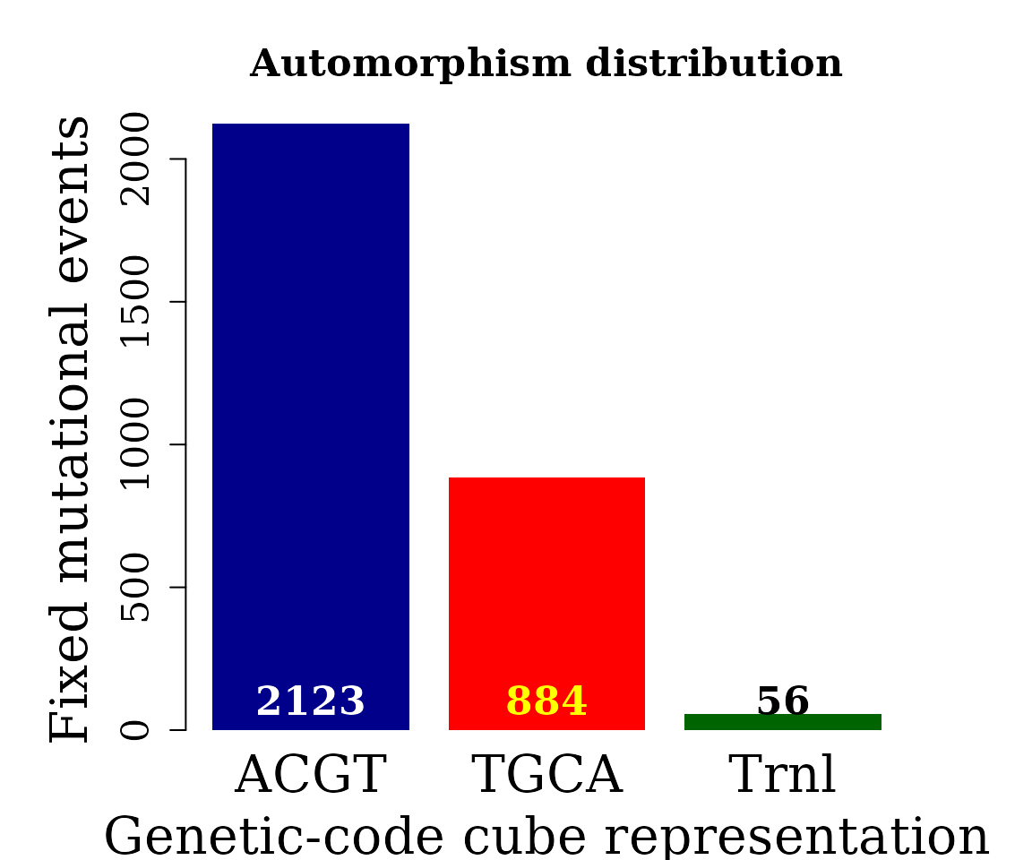
Analysis of conserved regions
conserv2 <- conserved_regions(x = covid_aut)
conserv2
#> AutomorphismByCoef object with 3813 ranges and 7 metadata columns:
#>          seqnames    ranges strand |        seq1        seq2         aa1         aa2      autm    mut_type        cube
#>             <Rle> <IRanges>  <Rle> | <character> <character> <character> <character> <numeric> <character> <character>
#>      [1]        1       1-4      + |         ATG         ATG           M           M         1         HHH        ACGT
#>      [2]        1       1-4      + |         GAG         GAG           E           E         1         HHH        ACGT
#>      [3]        1       1-4      + |         AGC         AGC           S           S         1         HHH        ACGT
#>      [4]        1       1-4      + |         CTT         CTT           L           L         1         HHH        ACGT
#>      [5]        1         7      + |         GGT         GGT           G           G         1         HHH        ACGT
#>      ...      ...       ...    ... .         ...         ...         ...         ...       ...         ...         ...
#>   [3809]        1 7093-7094      + |         GAT         GAT           D           D         1         HHH        ACGT
#>   [3810]        1 7096-7097      + |         CTT         CTT           L           L         1         HHH        ACGT
#>   [3811]        1 7096-7097      + |         GTT         GTT           V           V         1         HHH        ACGT
#>   [3812]        1 7099-7100      + |         AAC         AAC           N           N         1         HHH        ACGT
#>   [3813]        1 7099-7100      + |         TAA         TAA           *           *         1         HHH        ACGT
#>   -------
#>   seqinfo: 1 sequence from an unspecified genome; no seqlengths
Next, function fitCDF is applied to find the best fitted probability function to the the sizes of conserved regions.
widths <- width(conserv2)
dist2 <- fitCDF(widths, distNames = c(3, 7, 9, 10, 11, 12, 19, 20), plot = TRUE,
               loss.fun = "cauchy")
#>
#> *** Fitting Half-Normal distribution ...
#> .Fitting Done.
#>
#> *** Fitting Gamma distribution ...
#> .Fitting Done.
#>
#> *** Fitting Generalized 4P Gamma distribution ...
#> .Fitting Done.
#>
#> *** Fitting Generalized 3P Gamma distribution ...
#> .Fitting Done.
#>
#> *** Fitting Weibull distribution ...
#> .Fitting Done.
#>
#> *** Fitting 3P Weibull distribution ...
#> .Fitting Done.
#>
#> *** Fitting Exponential distribution ...
#> .Fitting Done.
#>
#> *** Fitting 2P Exponential distribution ...
#> .Fitting Done.
#>  * Estimating Studentized residuals for Generalized 4P Gamma distribution
#>  * Plots for Generalized 4P Gamma distribution...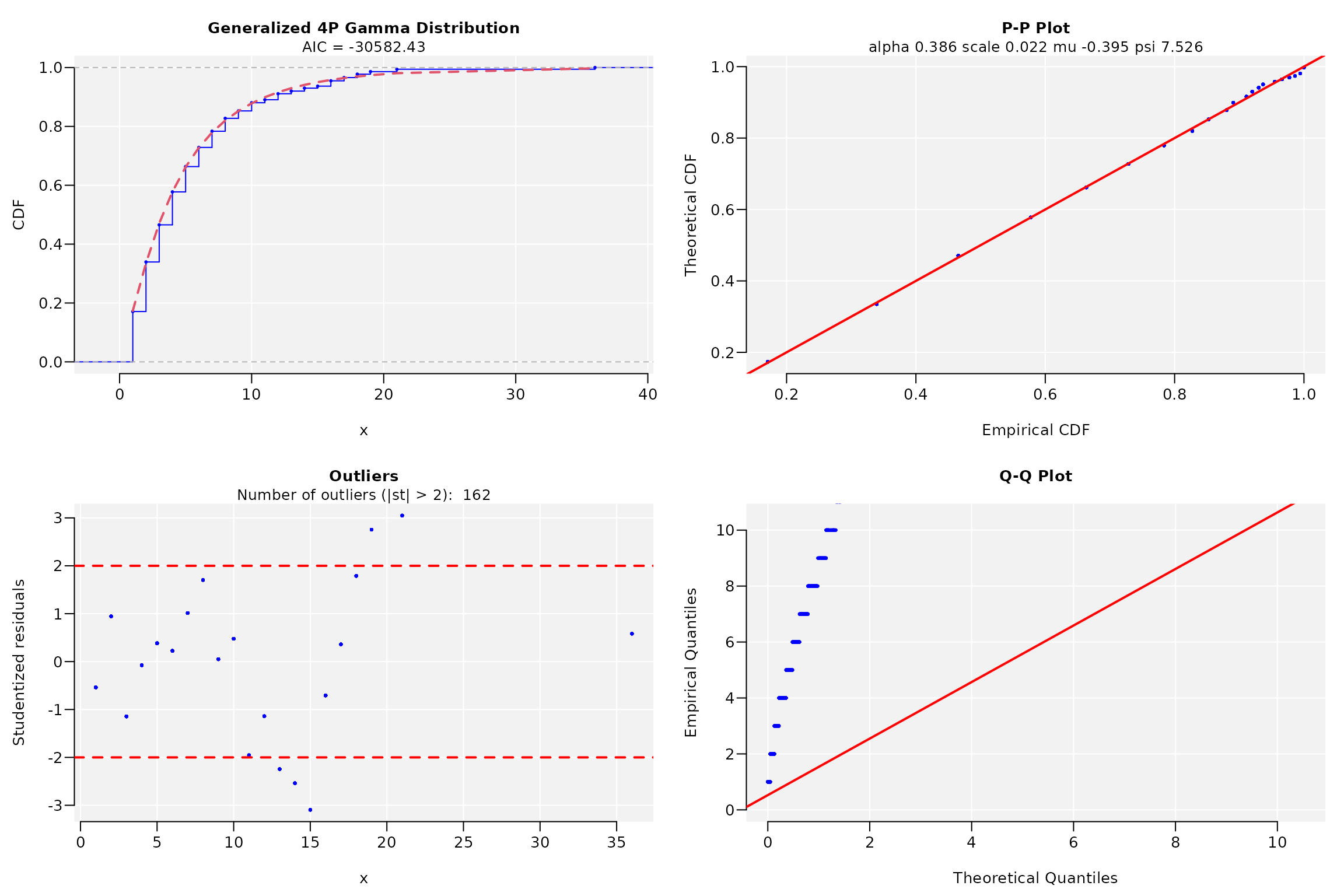
dist2
#> ggamma CDF model
#> ------
#> Parameters:
#>          Estimate  Std. Error   t value   Pr(>|t|)
#> alpha  0.38596938  0.01174701  32.85681 < 2.22e-16 ***
#> scale  0.02195697  0.00742671   2.95649  0.0031308 **
#> mu    -0.39511486  0.01856885 -21.27837 < 2.22e-16 ***
#> psi    7.52471426  0.52104576  14.44156 < 2.22e-16 ***
#> ---
#> Signif. codes:  0 '***' 0.001 '**' 0.01 '*' 0.05 '.' 0.1 ' ' 1
#>
#> Residual standard error: 1.809493e-05 on 3809 degrees of freedom
#> Number of iterations to termination: 222
#> Reason for termination: Relative error in the sum of squares is at most `ftol'.
#>
#> Goodness of fit:
#>     Adj.R.Square rho R.Cross.val       AIC
#> gof            1   1   0.9998617 -30582.48
par(lwd = 0.5, cex.axis = 2, cex.lab =1.4,
    cex.main = 2, mar=c(5,6,4,4), family = "serif")
hist(widths, 20, freq = FALSE, las = 1, family = "serif",
col = "cyan1", cex.main = 0.9,
main = "Histogram and best fitted CDF model for conserved region sizes",
xlab = "Conserved region size (bp)", yaxt = "n", ylab="", cex.axis = 1.4)
axis(side = 2, cex.axis = 1.4, las = 2)
mtext("Density", side = 2, cex = 1.4, line = 3.5)

x1 <- seq(1, 35, by = 1)
txt <- TeX(r'($\textit{f}(\textit{x}) = \frac{\alpha}{\beta\Gamma(\gamma)}
  {(\frac{\textit{x - \mu}}{\beta})}^{\alpha\delta-1}
  e^{(-\frac{\textit{x - \mu}}{\beta})^\alpha}$)')

lines(x1, dggamma(x1,
                  alpha = coef(dist2$bestfit)[1],
                  scale = coef(dist2$bestfit)[2],
                  mu = coef(dist2$bestfit)[3],
                  psi = coef(dist2$bestfit)[4]
                  ),
      col = "red", lwd = 1)
mtext(txt, side = 3, line = -4, cex = 1.4, adj = 0.7)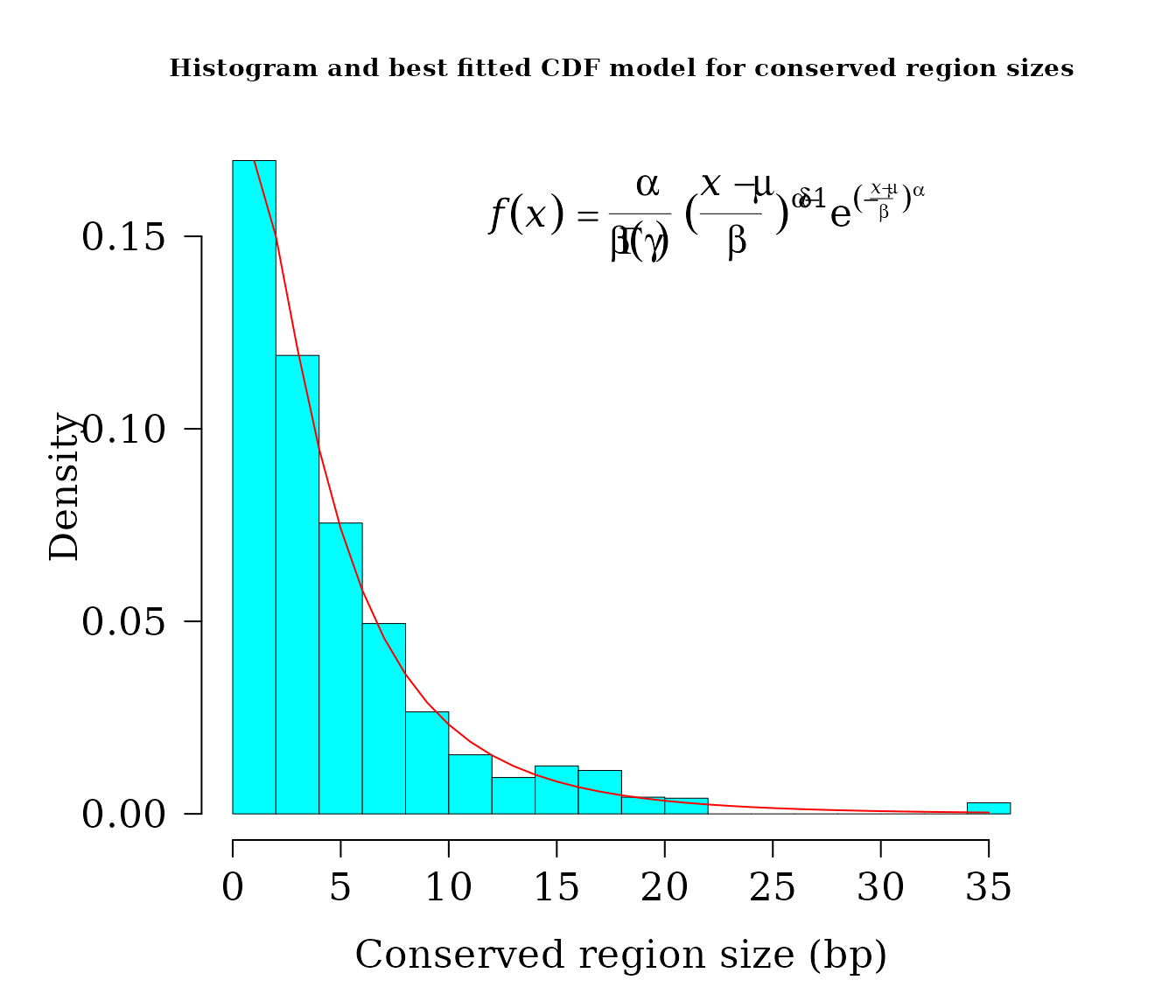
After apply Bootstrap test for Goodness of fit, tt seems to be that we have no reasons to reject the hypothesis that the sizes of conserved regions follows Generalized Gamma distribution.
mcgoftest(
          varobj = widths,
          model = dist2,
          stat = "ks")
#> *** Permutation GoF testing based on Kolmogorov-Smirnov statistic ( parametric approach )  ...
#>       KS.stat.D      mc_p.value KS.stat.p.value     sample.size       num.sampl
#>    1.733499e-01    1.000000e+00   5.983316e-100    3.813000e+03    9.990000e+02


mcgoftest(
          varobj = widths,
          model = dist2,
          stat = "ad")
#> *** Permutation GoF testing based on Anderson–Darling statistic ( parametric approach )  ...
#>     AD.stat  mc_p.value sample.size   num.sampl
#>    119.2847      1.0000   3813.0000    999.0000
Grouping automorphism by automorphism’s coefficients. Types of mutations
autby_coef2 <- automorphism_bycoef(covid_aut)
autby_coef2 <- autby_coef2[ autby_coef2$autm != 1 & autby_coef2$autm != -1  ]
Alignment gaps denoting indel mutations are labeled as “—”.
counts2 <- table(autby_coef2$mut_type)
counts2 <- sort(counts2, decreasing = TRUE)
count. <- counts2[ counts2 > 9 ]

par(family = "serif", cex.axis = 2, font = 2, las = 1,
    cex.main = 1.4, mar = c(6,3,4,4))
barplot(count., main="Automorphism distribution per Mutation type",
        col = colorRampPalette(c("red", "yellow", "blue"))(36),
        border = NA, axes = FALSE,las=2)
axis(side = 2,  cex.axis = 2, line = -1.8 )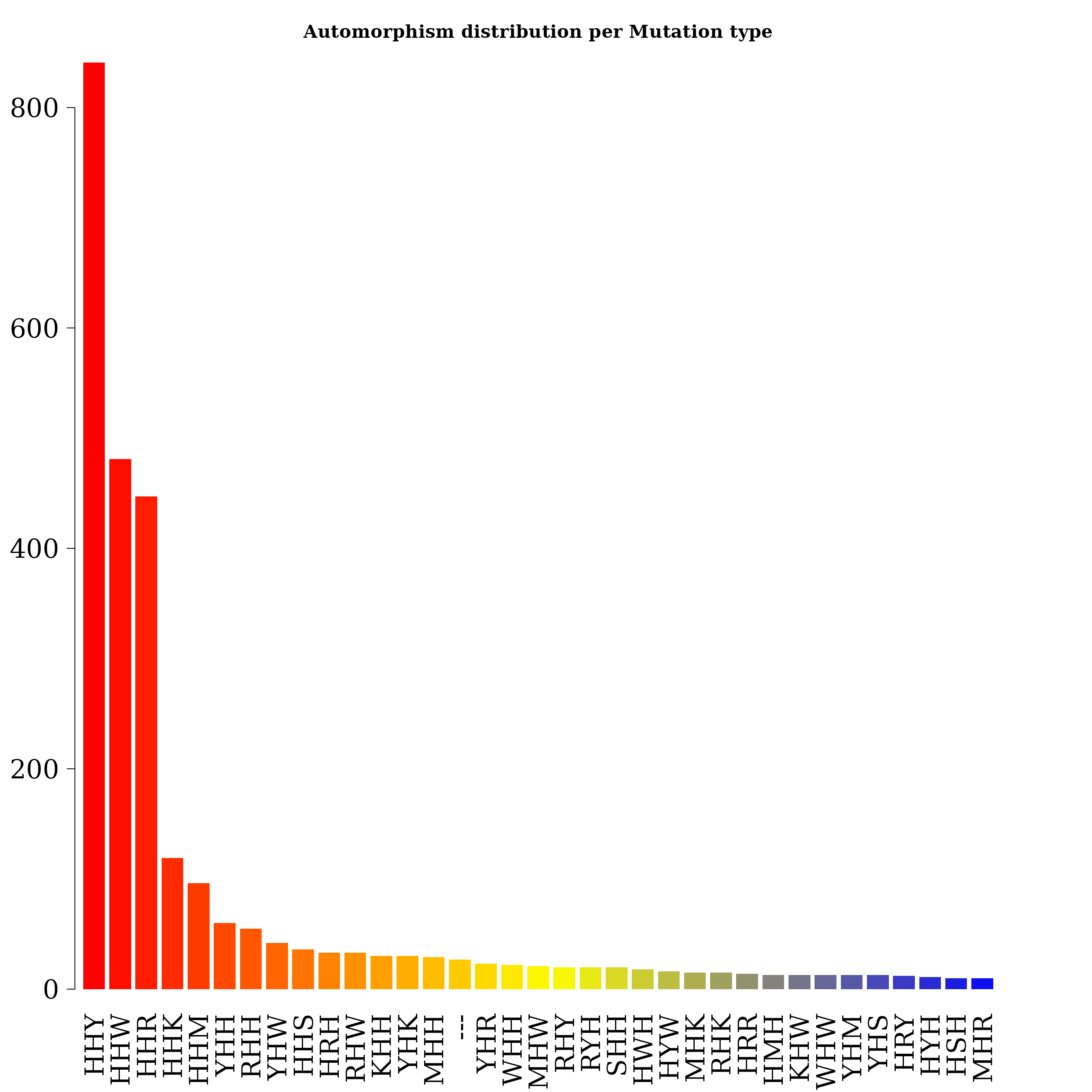
counts2
#>
#> HHY HHW HHR HHK HHM YHH RHH YHW HHS HRH RHW KHH YHK MHH --- YHR WHH MHW RHY RYH SHH HWH HYW MHK RHK HRR HMH KHW WHW YHM
#> 841 481 447 119  96  60  55  42  36  33  33  30  30  29  27  23  22  21  20  20  20  18  16  15  15  14  13  13  13  13
#> YHS HRY HYH HSH MHR HMW HWY HYY MHY SHR WHR HKY HMY RHR SHK WHM KHY KSH MHM RMH RRW RRY WSH KYH RMW RRH SHM SHW SHY YHY
#>  13  12  11  10  10   9   9   9   9   9   9   7   7   7   7   7   6   6   6   6   6   6   6   5   5   5   5   5   5   5
#> HKH HMR HSW HYR MRW RHM RYM WHK HKW HWK HWW HYM KHK KHM KHR KHS MMR MYH RHS RMR RRK RWW RYW RYY SMH WHY WSM HMK HMM HRK
#>   4   4   4   4   4   4   4   4   3   3   3   3   3   3   3   3   3   3   3   3   3   3   3   3   3   3   3   2   2   2
#> HSY HWM KMH KSM KWH MHS MMH MMM MMW MRH MRK RMY RSY RWK RWR RYK SYH WHS WKK WYK WYW YSH HMS HRM HRW HSK HWR HYK HYS KKK
#>   2   2   2   2   2   2   2   2   2   2   2   2   2   2   2   2   2   2   2   2   2   2   1   1   1   1   1   1   1   1
#> KMW KSW KWW KWY KYK KYW KYY MKH MSM MWH MWM MYK MYM MYR MYW RKH RKW RMK RRS RSH RSW RWY RYR SHS SKW SMK SMS SMW SRH SRM
#>   1   1   1   1   1   1   1   1   1   1   1   1   1   1   1   1   1   1   1   1   1   1   1   1   1   1   1   1   1   1
#> SWK SWM SWS SWW SYW WKH WKM WMH WMK WMW WMY WRH WSW WSY WWH WWY WYM WYR WYS YKH YKR YMH YMM YMS YMW YRH YWH YWM YWS YWY
#>   1   1   1   1   1   1   1   1   1   1   1   1   1   1   1   1   1   1   1   1   1   1   1   1   1   1   1   1   1   1
#> YYH
#>   1
SARS coronavirus GZ02 vs bat-SL-CoVZC45 and Bat SARS-like coronavirus isolate Rs7327
data(covid_autm, package = "GenomAutomorphism")
covid_autm
#> Automorphism object with 9722 ranges and 8 metadata columns:
#>          seqnames    ranges strand |        seq1        seq2         aa1         aa2    coord1    coord2      autm
#>             <Rle> <IRanges>  <Rle> | <character> <character> <character> <character> <numeric> <numeric> <numeric>
#>      [1]        1         1      + |         ATG         ATG           M           M        50        50         1
#>      [2]        1         2      + |         GAG         GAG           E           E        10        10         1
#>      [3]        1         3      + |         AGC         AGC           S           S        33        33         1
#>      [4]        1         4      + |         CTT         CTT           L           L        55        55         1
#>      [5]        1         5      + |         GTT         GTT           V           V        59        59         1
#>      ...      ...       ...    ... .         ...         ...         ...         ...       ...       ...       ...
#>   [9718]        1      9718      + |         TCA         TCA           S           S        28        28         1
#>   [9719]        1      9719      + |         ACT         ACT           T           T        19        19         1
#>   [9720]        1      9720      + |         CAG         CAG           Q           Q         6         6         1
#>   [9721]        1      9721      + |         GCA         GCA           A           A        24        24         1
#>   [9722]        1      9722      + |         TAA         TAA           *           *        12        12         1
#>                 cube
#>          <character>
#>      [1]        ACGT
#>      [2]        ACGT
#>      [3]        ACGT
#>      [4]        ACGT
#>      [5]        ACGT
#>      ...         ...
#>   [9718]        ACGT
#>   [9719]        ACGT
#>   [9720]        ACGT
#>   [9721]        ACGT
#>   [9722]        ACGT
#>   -------
#>   seqinfo: 1 sequence from an unspecified genome; no seqlengths
conserv <- conserved_regions(covid_autm)
conserv
#> AutomorphismByCoef object with 6348 ranges and 7 metadata columns:
#>          seqnames    ranges strand |        seq1        seq2         aa1         aa2      autm    mut_type        cube
#>             <Rle> <IRanges>  <Rle> | <character> <character> <character> <character> <numeric> <character> <character>
#>      [1]        1      1-19      + |         ATG         ATG           M           M         1         HHH        ACGT
#>      [2]        1      1-19      + |         GAG         GAG           E           E         1         HHH        ACGT
#>      [3]        1      1-19      + |         AGC         AGC           S           S         1         HHH        ACGT
#>      [4]        1      1-19      + |         CTT         CTT           L           L         1         HHH        ACGT
#>      [5]        1      1-19      + |         GTT         GTT           V           V         1         HHH        ACGT
#>      ...      ...       ...    ... .         ...         ...         ...         ...       ...         ...         ...
#>   [6344]        1 9683-9722      + |         GGA         GGA           G           G         1         HHH        ACGT
#>   [6345]        1 9683-9722      + |         TCT         TCT           S           S         1         HHH        ACGT
#>   [6346]        1 9683-9722      + |         TCA         TCA           S           S         1         HHH        ACGT
#>   [6347]        1 9683-9722      + |         GCA         GCA           A           A         1         HHH        ACGT
#>   [6348]        1 9683-9722      + |         TAA         TAA           *           *         1         HHH        ACGT
#>   -------
#>   seqinfo: 1 sequence from an unspecified genome; no seqlengths
consvr <- c(conserv, conserv2)
widths <- width(consvr)
dist <- fitCDF(widths, distNames = c(2, 3, 7, 9, 10, 11, 19, 20), plot = TRUE,
               loss.fun = "cauchy")
#>
#> *** Fitting Log-normal distribution ...
#> .Fitting Done.
#>
#> *** Fitting Half-Normal distribution ...
#> .Fitting Done.
#>
#> *** Fitting Gamma distribution ...
#> .Fitting Done.
#>
#> *** Fitting Generalized 4P Gamma distribution ...
#> .Fitting Done.
#>
#> *** Fitting Generalized 3P Gamma distribution ...
#> .Fitting Done.
#>
#> *** Fitting Weibull distribution ...
#> .Fitting Done.
#>
#> *** Fitting Exponential distribution ...
#> .Fitting Done.
#>
#> *** Fitting 2P Exponential distribution ...
#> .Fitting Done.
#>  * Estimating Studentized residuals for Generalized 4P Gamma distribution
#>  * Plots for Generalized 4P Gamma distribution...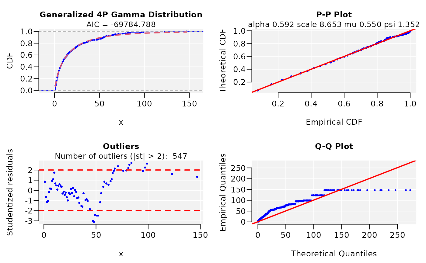
dist
#> ggamma CDF model
#> ------
#> Parameters:
#>          Estimate  Std. Error   t value   Pr(>|t|)
#> alpha 0.591610381 0.003539813 167.13041 < 2.22e-16 ***
#> scale 8.652891132 0.218974837  39.51546 < 2.22e-16 ***
#> mu    0.549870141 0.005491076 100.13888 < 2.22e-16 ***
#> psi   1.352270767 0.015700233  86.13062 < 2.22e-16 ***
#> ---
#> Signif. codes:  0 '***' 0.001 '**' 0.01 '*' 0.05 '.' 0.1 ' ' 1
#>
#> Residual standard error: 5.502277e-05 on 10157 degrees of freedom
#> Number of iterations to termination: 24
#> Reason for termination: Relative error in the sum of squares is at most `ftol'.
#>
#> Goodness of fit:
#>     Adj.R.Square rho R.Cross.val       AIC
#> gof            1   1   0.9996438 -69784.96
Joining the datasets increases the sample size and improved predictions in respect to the comparison SARS coronavirus GZ02 vs Bat SARS-like coronavirus alone.
par(lwd = 0.5, cex.axis = 2, cex.lab =1.4,
    cex.main = 2, mar=c(5,6,4,4), family = "serif")
hist(widths, 14, freq = FALSE, las = 1, family = "serif",
col = "cyan1", cex.main = 0.9,
main = "Histogram and best fitted CDF model for conserved region sizes",
xlab = "Conserved region size (bp)", yaxt = "n", ylab="", cex.axis = 1.4)
axis(side = 2, cex.axis = 1.4, las = 2)
mtext("Density", side = 2, cex = 1.4, line = 3.5)

x1 <- seq(1, 150, by = 1)
txt <- TeX(r'($\textit{f}(\textit{x}) = \frac{\alpha}{\beta\Gamma(\gamma)}
  {(\frac{\textit{x - \mu}}{\beta})}^{\alpha\delta-1}
  e^{(-\frac{\textit{x - \mu}}{\beta})^\alpha}$)')

lines(x1, dggamma(x1,
                  alpha = coef(dist$bestfit)[1],
                  scale = coef(dist$bestfit)[2],
                  psi = coef(dist$bestfit)[3]
                  ),
      col = "red", lwd = 1)
mtext(txt, side = 3, line = -4, cex = 1.4, adj = 0.7)
mcgoftest(
          varobj = widths,
          model = dist,
          stat = "ks")
#> *** Permutation GoF testing based on Kolmogorov-Smirnov statistic ( parametric approach )  ...
#>       KS.stat.D      mc_p.value KS.stat.p.value     sample.size       num.sampl
#>    8.628456e-02    1.000000e+00    3.919415e-66    1.016100e+04    9.990000e+02

cat("\n===========================\n")
#>
#> ===========================
mcgoftest(
          varobj = widths,
          model = dist,
          stat = "ad")
#> *** Permutation GoF testing based on Anderson–Darling statistic ( parametric approach )  ...
#>     AD.stat  mc_p.value sample.size   num.sampl
#>    70.64955     1.00000 10161.00000   999.00000
Grouping automorphism by automorphism’s coefficients
autby_coef <- automorphism_bycoef(covid_autm)
autby_coef <- c(autby_coef, autby_coef2)
autby_coef <- autby_coef[ autby_coef$autm != 1 & autby_coef$autm != -1  ]
Alignment gaps denoting indel mutations are labeled as “—”.
counts <- table(autby_coef$mut_type)
counts <- sort(counts, decreasing = TRUE)
count. <- counts[ counts > 9 ]

par(family = "serif", cex.axis = 2, font = 2, las = 1,
    cex.main = 1.4, cex.lab = 2, mar = c(6,4,4,1))
barplot(count., main="Automorphism distribution per Mutation type",
        col = colorRampPalette(c("red", "yellow", "blue"))(36),
        border = NA, axes = FALSE,las=2)
axis(side = 2,  cex.axis = 2, line = -1.8 )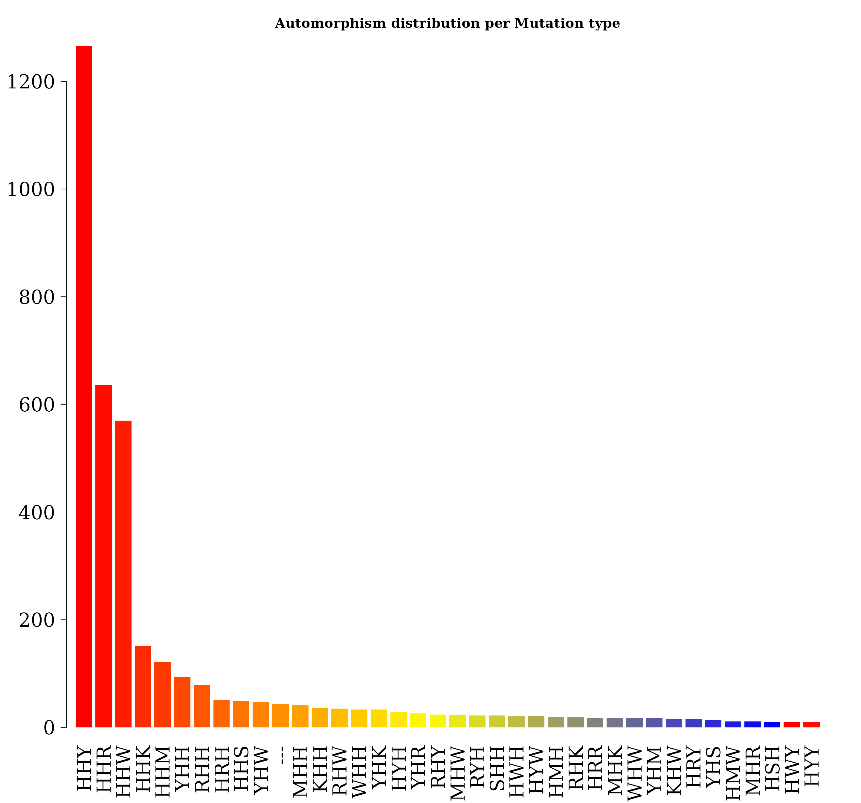
counts
#>
#>  HHY  HHR  HHW  HHK  HHM  YHH  RHH  HRH  HHS  YHW  ---  MHH  KHH  RHW  WHH  YHK  HYH  YHR  RHY  MHW  RYH  SHH  HWH  HYW
#> 1266  636  570  151  121   94   79   51   49   47   43   41   36   35   33   33   29   26   24   23   22   22   21   21
#>  HMH  RHK  HRR  MHK  WHW  YHM  KHW  HRY  YHS  HMW  MHR  HSH  HWY  HYY  MHY  RHR  SHR  WHR  YHY  HMY  KHY  RMH  RRY  HKH
#>   20   19   17   17   17   17   16   15   14   11   11   10   10   10    9    9    9    9    9    8    8    8    8    7
#>  HKY  HMR  KSH  RMW  SHK  SHW  WHM  MHM  RHM  RRW  RYY  SHM  SHY  WSH  HYR  KYH  RRH  RYW  HSW  HWW  KHK  KHR  MRH  MRW
#>    7    7    7    7    7    7    7    6    6    6    6    6    6    6    5    5    5    5    4    4    4    4    4    4
#>  RRK  RYM  WHK  WHY  HKW  HMK  HWK  HYK  HYM  KHM  KHS  KMH  KSW  MHS  MMM  MMR  MYH  RHS  RKW  RMR  RMY  RSW  RWW  RYK
#>    4    4    4    4    3    3    3    3    3    3    3    3    3    3    3    3    3    3    3    3    3    3    3    3
#>  SMH  SRH  SYH  WMH  WSM  WSY  WYW  YWH  HMM  HRK  HSY  HWM  KMW  KSM  KWH  MMH  MMW  MRK  MWH  MWM  RSY  RWK  RWR  SMW
#>    3    3    3    3    3    3    3    3    2    2    2    2    2    2    2    2    2    2    2    2    2    2    2    2
#>  SRM  WHS  WKK  WMS  WRH  WWH  WWY  WYK  WYM  YKH  YSH  YWM  YWY  YYH  HKK  HKR  HMS  HRM  HRW  HSK  HSR  HWR  HWS  HYS
#>    2    2    2    2    2    2    2    2    2    2    2    2    2    2    1    1    1    1    1    1    1    1    1    1
#>  KKK  KKS  KRK  KRY  KWW  KWY  KYK  KYW  KYY  MKH  MKM  MRM  MSM  MWS  MWW  MYK  MYM  MYR  MYW  MYY  RKH  RMK  RRM  RRS
#>    1    1    1    1    1    1    1    1    1    1    1    1    1    1    1    1    1    1    1    1    1    1    1    1
#>  RSH  RSK  RWY  RYR  SHS  SKW  SKY  SMK  SMS  SWK  SWM  SWR  SWS  SWW  SWY  SYW  WKH  WKM  WMK  WMW  WMY  WRY  WSW  WWK
#>    1    1    1    1    1    1    1    1    1    1    1    1    1    1    1    1    1    1    1    1    1    1    1    1
#>  WWS  WYH  WYR  WYS  YKR  YKY  YMH  YMM  YMS  YMW  YRH  YRY  YWS  YWW  YYR
#>    1    1    1    1    1    1    1    1    1    1    1    1    1    1    1