
Get started with GenomAutomorphism
Robersy Sanchez
EpiMethyl Analytics, 10401 Baur Blvd, Suite F, St. Louis, MO 63132
genomicmath@gmail.com
01 August 2026
Source:vignettes/GenomAutomorphism.Rmd
GenomAutomorphism.RmdAbstract
A fast introduction into the analysis of DNA mutational events by means of automorphisms between two DNA sequences algebraically represented as Abelian finite group.
GenomAutomorphism Overview
This is an R package to compute the automorphisms between pairwise aligned DNA sequences represented as elements from a Genomic Abelian group as described in reference (1). In a general scenario, whole chromosomes or genomic regions from a population (from any species or closely related species) can be algebraically represented as a direct sum of cyclic groups or more specifically Abelian p-groups. Basically, we propose the representation of multiple sequence alignments (MSA) of length N as a finite Abelian group created by the direct sum of Abelian groups of prime-power order:
Where, the ’s are prime numbers, and is the group of integer modulo .
For the purpose of estimating the automorphism between two aligned DNA sequences, .
Installing GenomAutomorphism
GenomAutomorphism uses several R dependencies, which can
be installed as follows:
if (!requireNamespace("BiocManager"))
    install.packages("BiocManager")

BiocManager::install(c("Biostrings", "GenomicRanges", "S4Vectors",
        "BiocParallel", "Seqinfo", "BiocGenerics", "numbers", "devtools",
        "doParallel", "data.table", "foreach","parallel"), dependencies = TRUE)
GenomAutomorphism can be installed as follows:
if (!require("BiocManager", quietly = TRUE))
    install.packages("BiocManager")

BiocManager::install("GenomAutomorphism")
You can install the GenomAutomorphism package from
GitHub as follows
BiocManager::install('genomaths/GenomAutomorphism')You can install the GenomAutomorphism ‘beta’ package
with the latest updates (which may differ from the Bioconductor version)
from GitHub as follows:
BiocManager::install('genomaths/GenomAutomorphism_beta')Automorphisms
Herein, automorphisms are considered algebraic descriptions of mutational events observed in codon sequences represented on different Abelian groups. In particular, as described in references (3-4), for each representation of the codon set on a defined Abelian group there are 24 possible isomorphic Abelian groups. These Abelian groups can be labeled based on the DNA base-order used to generate them. The set of 24 Abelian groups can be described as a group isomorphic to the symmetric group of degree four (, see reference (4)).
For further support about the symmetric group on the 24 Abelian groups of genetic-code cubes, users can also see Symmetric Group of the Genetic-Code Cubes., specifically the Mathematica notebook IntroductionToZ5GeneticCodeVectorSpace.nb and interact with it using Wolfram Player, freely available (for Windows and Linux OS) at, https://www.wolfram.com/player/.
Read the FASTA alignment and encode the sequences
A pairwise sequence alignment of protein-coding regions of SARS coronavirus GZ02 (GenBank: AY390556.1) and Bat SARS-like coronavirus isolate Rs7327 (GenBank: KY417151.1) is provided with the package.
data(covid_aln, package = "GenomAutomorphism")
covid_aln
#> DNAMultipleAlignment with 2 rows and 29166 columns
#>      aln                                                                                            names
#> [1] ATGGAGAGCCTTGTTCTTGGTGTCAACGAGAAAACACACGTCCAAC...CAAAATTCCATGAGTGGAGCTTCTGCTGATTCAACTCAGGCATAA lcl|AY390556.1_cd...
#> [2] ATGGAGAGCCTTGTTCTTGGTGTCAACGAGAAAACACACGTCCAAC...CAAAATTCCATGAGTGGAGCTTCTGCTGATTCAACTCAGGCATAA lcl|KY417151.1_cd...
Group representations
Group operations defined on the sets of DNA bases and codons are associated with physicochemical and/or biophysical relationships between DNA bases and between codons and aminoacids. In other words, a proper definition of a group operation on the set of bases or on the set of codons will encode the physicochemical and/or biophysical relationships between the set’s elements. Thus, by group operations defined on the set of bases or on the set of codons, we understand an encoding applied to represent specified physicochemical and/or biophysical relationships as group operations between the elements of the set. Then, we shall say that such an encoding permits the representation of DNA bases, codons, genes, and genomic sequences as elements from algebraic structures.
The DNA base set can be represented in 24 possible base orders, which leads to 24 possible representations of the genetic code. Each genetic code representation of base-triplets on the Galois field GF(4) (or in GF(5)) leads to a genetic-code vector 3D-space, which is mathematically equivalent to a cube inserted in the 3D space (1). Each cube is denoted according to the corresponding base order.
Given a base-order, say ‘ACGT’, the Abelian group defined on this ordered set is isomorphic to the Abelian group defined on the set of integers modulo 4 (). In practical terms, this is equivalent to replacing each DNA base by the corresponding integer element. The base replacement in cube “ACGT” and group “Z4” () is:
base2int("ACGT", group = "Z4", cube = "ACGT")
#> [1] 0 1 2 3
The base replacement in cube “ACGT” and group “Z5” ():
base2int("ACGT", group = "Z5", cube = "ACGT")
#> [1] 1 2 3 4
After the DNA sequence is read, the corresponding codon sequences can be represented in the Abelian group (i.e., the set of integers remainder modulo 64). The codon coordinates are requested on the cube ACGT. Following reference (4), cubes are labeled based on the order of DNA bases used to define the sum operation.
codons <- codon_coord(
                    codon = covid_aln,
                    cube = "ACGT",
                    group = "Z64",
                    chr = 1L,
                    strand = "+",
                    start = 1,
                    end = 750)
codons
#> CodonGroup object with 250 ranges and 4 metadata columns:
#>         seqnames    ranges strand |        seq1        seq2      coord1      coord2
#>            <Rle> <IRanges>  <Rle> | <character> <character> <character> <character>
#>     [1]        1         1      + |         ATG         ATG          50          50
#>     [2]        1         2      + |         GAG         GAG          10          10
#>     [3]        1         3      + |         AGC         AGC          33          33
#>     [4]        1         4      + |         CTT         CTT          55          55
#>     [5]        1         5      + |         GTT         GTT          59          59
#>     ...      ...       ...    ... .         ...         ...         ...         ...
#>   [246]        1       246      + |         GAT         GAT          11          11
#>   [247]        1       247      + |         AAG         AAG           2           2
#>   [248]        1       248      + |         AGC         AGC          33          33
#>   [249]        1       249      + |         TAC         TAT          13          15
#>   [250]        1       250      + |         GAG         GAG          10          10
#>   -------
#>   seqinfo: 1 sequence from an unspecified genome; no seqlengths
The codon sequences (seq1 and seq2) with their corresponding coordinates (left) are returned, as well as the coordinate representation on (coord1 and coord2).
“Dual” genetic-code cubes
Of particular interest is the coordinate representation on “dual” genetic-code cubes. These are cubes where codons with complementary base pairs have the same coordinates in the corresponding cubes, as shown in reference (4). Each pair of “dual” cubes integrates a group.
For example, let’s consider the complementary codons “ACG” and “TGC”, with complementary base pairs: A::T, C:::G, and G:::C, where symbol “:” denotes the hydrogen bonds between the bases.
x0 <- c("ACG", "TGC")
x1 <- DNAStringSet(x0)
x1
#> DNAStringSet object of length 2:
#>     width seq
#> [1]     3 ACG
#> [2]     3 TGC
Their representations on the dual cubes “ACGT” and “TGCA” on are:
x2 <- base_coord(x1, cube = "ACGT")
x2
#> BaseGroup object with 3 ranges and 4 metadata columns:
#>       seqnames    ranges strand |        seq1        seq2    coord1    coord2
#>          <Rle> <IRanges>  <Rle> | <character> <character> <numeric> <numeric>
#>   [1]        1         1      + |           A           T         0         3
#>   [2]        1         2      + |           C           G         1         2
#>   [3]        1         3      + |           G           C         2         1
#>   -------
#>   seqinfo: 1 sequence from an unspecified genome; no seqlengths

x2. <- base_coord(x1, cube = "TGCA")
x2.
#> BaseGroup object with 3 ranges and 4 metadata columns:
#>       seqnames    ranges strand |        seq1        seq2    coord1    coord2
#>          <Rle> <IRanges>  <Rle> | <character> <character> <numeric> <numeric>
#>   [1]        1         1      + |           A           T         3         0
#>   [2]        1         2      + |           C           G         2         1
#>   [3]        1         3      + |           G           C         1         2
#>   -------
#>   seqinfo: 1 sequence from an unspecified genome; no seqlengths
The sum of base coordinates modulo is 3.
## cube "ACGT"
(x2$coord1 + x2$coord2) %% 4
#> [1] 3 3 3

## cube "TGCA"
(x2.$coord1 + x2.$coord2) %% 4
#> [1] 3 3 3
The same result for the same codon on different cubes.
## Codon ACG
(x2$coord1 + x2.$coord1) %% 4
#> [1] 3 3 3

## Codon TGC
(x2$coord2 + x2.$coord2) %% 4
#> [1] 3 3 3
Their codon representations on are:
## cube ACGT
x3 <- codon_coord(codon = x2, group = "Z64")
x3
#> CodonGroup object with 1 range and 4 metadata columns:
#>       seqnames    ranges strand |        seq1        seq2      coord1      coord2
#>          <Rle> <IRanges>  <Rle> | <character> <character> <character> <character>
#>   [1]        1         1      + |         ACG         TGC          18          45
#>   -------
#>   seqinfo: 1 sequence from an unspecified genome; no seqlengths

## cube TGCA
x3. <- codon_coord(codon = x2., group = "Z64")
x3.
#> CodonGroup object with 1 range and 4 metadata columns:
#>       seqnames    ranges strand |        seq1        seq2      coord1      coord2
#>          <Rle> <IRanges>  <Rle> | <character> <character> <character> <character>
#>   [1]        1         1      + |         ACG         TGC          45          18
#>   -------
#>   seqinfo: 1 sequence from an unspecified genome; no seqlengths
The sum of base coordinates modulo is 63.
## cube "ACGT"
(as.numeric(x3$coord1) + as.numeric(x3$coord2)) %% 64
#> [1] 63

## cube "TGCA"
(as.numeric(x3.$coord1) + as.numeric(x3.$coord2)) %% 64
#> [1] 63
The same result for the same codon on different cubes.
## Codon ACG
(as.numeric(x3$coord1) + as.numeric(x3.$coord1)) %% 64
#> [1] 63

## Codon TGC
(as.numeric(x3$coord2) + as.numeric(x3.$coord2)) %% 64
#> [1] 63
Automorphisms on
Automorphisms can be computed starting directly from the FASTA file. Notice that we can work only with genomic regions of interest by giving the start and end alignment coordinates. In automorphisms are described as functions , where and are elements from the set of integers modulo 64. Below, in function automorphisms three important arguments are given values: group = “Z64”, cube = c(“ACGT”, “TGCA”), and cube_alt = c(“CATG”, “GTAC”).
In groups
and
,
not all the mutational events can be described as automorphisms from a
given cube. The analysis of automorphisms is then accomplished in the
set of dual genetic-code cubes. A character string denoting
pairs of dual genetic-code cubes is given as the argument for
cube. The group setting specifies on which group the
automorphisms will be computed. These groups can be:
(group = "Z5"),
(group = "Z64"),
(group = "Z125"), and
(group = "Z5^3").
If automorphisms are not found in the first set of dual cubes, then the algorithm searches for automorphisms in an alternative set of dual cubes.
autm <- automorphisms(
                    seqs = covid_aln,
                    group = "Z64",
                    cube = c("ACGT", "TGCA"),
                    cube_alt = c("CATG", "GTAC"),
                    start = 1,
                    end = 750,
                    verbose = FALSE)
autm
#> Automorphism object with 250 ranges and 8 metadata columns:
#>         seqnames    ranges strand |        seq1        seq2         aa1         aa2    coord1    coord2      autm
#>            <Rle> <IRanges>  <Rle> | <character> <character> <character> <character> <numeric> <numeric> <numeric>
#>     [1]        1         1      + |         ATG         ATG           M           M        50        50         1
#>     [2]        1         2      + |         GAG         GAG           E           E        10        10         1
#>     [3]        1         3      + |         AGC         AGC           S           S        33        33         1
#>     [4]        1         4      + |         CTT         CTT           L           L        55        55         1
#>     [5]        1         5      + |         GTT         GTT           V           V        59        59         1
#>     ...      ...       ...    ... .         ...         ...         ...         ...       ...       ...       ...
#>   [246]        1       246      + |         GAT         GAT           D           D        11        11         1
#>   [247]        1       247      + |         AAG         AAG           K           K         2         2         1
#>   [248]        1       248      + |         AGC         AGC           S           S        33        33         1
#>   [249]        1       249      + |         TAC         TAT           Y           Y        13        15        11
#>   [250]        1       250      + |         GAG         GAG           E           E        10        10         1
#>                cube
#>         <character>
#>     [1]        ACGT
#>     [2]        ACGT
#>     [3]        ACGT
#>     [4]        ACGT
#>     [5]        ACGT
#>     ...         ...
#>   [246]        ACGT
#>   [247]        ACGT
#>   [248]        ACGT
#>   [249]        ACGT
#>   [250]        ACGT
#>   -------
#>   seqinfo: 1 sequence from an unspecified genome; no seqlengths
Observe that two new columns were added, the automorphism coefficient (named as autm) and the genetic-code cube where the automorphism was found. By convention, the DNA sequence is given for the positive strand. Since the dual cube of “ACGT” corresponds to the complementary base order TGCA, automorphisms described by the cube TGCA represent mutational events affecting the DNA negative strand (-).
The last result can be summarized by gene regions as follows:
aut_range <- automorphismByRanges(autm)
aut_range
#> GRanges object with 9 ranges and 1 metadata column:
#>       seqnames    ranges strand |        cube
#>          <Rle> <IRanges>  <Rle> | <character>
#>   [1]        1     1-102      + |        ACGT
#>   [2]        1       103      - |        TGCA
#>   [3]        1   104-105      + |        ACGT
#>   [4]        1       106      - |        TGCA
#>   [5]        1   107-201      + |        ACGT
#>   [6]        1       202      - |        TGCA
#>   [7]        1   203-205      + |        ACGT
#>   [8]        1       206      - |        TGCA
#>   [9]        1   207-250      + |        ACGT
#>   -------
#>   seqinfo: 1 sequence from an unspecified genome; no seqlengths
That is, function automorphismByRanges permits the classification of the pairwise alignment of protein-coding sub-regions based on the mutational events observed in it, quantitatively represented as automorphisms on genetic-code cubes.
Searching for automorphisms on allows a quantitative differentiation between mutational events at different codon positions from a given DNA protein-encoding region. As shown in reference (4), a set of different cubes can be applied to describe the best evolutionary aminoacid scale highly correlated with aminoacid physicochemical properties describing the observed evolutionary process in a given protein.
More information about this subject can be found in the supporting material from reference (4) at GitHub GenomeAlgebra_SymmetricGroup, particularly by interacting with the Mathematica notebook Genetic-Code-Scales_of_Amino-Acids.nb.
Automorphisms between whole genomes of SARS-CoV-2 related coronaviruses
Next, the automorphisms for the whole pairwise alignment of the SARS-CoV-2 related coronaviruses:
## Do not need to run it.
covid_autm <- automorphisms(
                    seqs = covid_aln,
                    group = "Z64",
                    cube = c("ACGT", "TGCA"),
                    cube_alt = c("CATG", "GTAC"),
                    verbose = FALSE)
This data is available with the package
data(covid_autm, package = "GenomAutomorphism")
covid_autm
#> Automorphism object with 9722 ranges and 8 metadata columns:
#>          seqnames    ranges strand |        seq1        seq2         aa1         aa2    coord1    coord2      autm
#>             <Rle> <IRanges>  <Rle> | <character> <character> <character> <character> <numeric> <numeric> <numeric>
#>      [1]        1         1      + |         ATG         ATG           M           M        50        50         1
#>      [2]        1         2      + |         GAG         GAG           E           E        10        10         1
#>      [3]        1         3      + |         AGC         AGC           S           S        33        33         1
#>      [4]        1         4      + |         CTT         CTT           L           L        55        55         1
#>      [5]        1         5      + |         GTT         GTT           V           V        59        59         1
#>      ...      ...       ...    ... .         ...         ...         ...         ...       ...       ...       ...
#>   [9718]        1      9718      + |         TCA         TCA           S           S        28        28         1
#>   [9719]        1      9719      + |         ACT         ACT           T           T        19        19         1
#>   [9720]        1      9720      + |         CAG         CAG           Q           Q         6         6         1
#>   [9721]        1      9721      + |         GCA         GCA           A           A        24        24         1
#>   [9722]        1      9722      + |         TAA         TAA           *           *        12        12         1
#>                 cube
#>          <character>
#>      [1]        ACGT
#>      [2]        ACGT
#>      [3]        ACGT
#>      [4]        ACGT
#>      [5]        ACGT
#>      ...         ...
#>   [9718]        ACGT
#>   [9719]        ACGT
#>   [9720]        ACGT
#>   [9721]        ACGT
#>   [9722]        ACGT
#>   -------
#>   seqinfo: 1 sequence from an unspecified genome; no seqlengths
And the summary by range
aut_range <- automorphismByRanges(covid_autm)
aut_range
#> GRanges object with 460 ranges and 1 metadata column:
#>         seqnames    ranges strand |        cube
#>            <Rle> <IRanges>  <Rle> | <character>
#>     [1]        1     1-102      + |        ACGT
#>     [2]        1       103      - |        TGCA
#>     [3]        1   104-105      + |        ACGT
#>     [4]        1       106      - |        TGCA
#>     [5]        1   107-201      + |        ACGT
#>     ...      ...       ...    ... .         ...
#>   [456]        1 9577-9608      + |        ACGT
#>   [457]        1      9609      - |        TGCA
#>   [458]        1 9610-9674      + |        ACGT
#>   [459]        1      9675      - |        TGCA
#>   [460]        1 9676-9722      + |        ACGT
#>   -------
#>   seqinfo: 1 sequence from an unspecified genome; no seqlengths
Regions not described by automorphisms can be described as translations (labeled “Trnl”) and they can be shown as follows:
idx = which(covid_autm$cube == "Trnl")
covid_autm[ idx ]
#> Automorphism object with 19 ranges and 8 metadata columns:
#>        seqnames    ranges strand |        seq1        seq2         aa1         aa2    coord1    coord2      autm
#>           <Rle> <IRanges>  <Rle> | <character> <character> <character> <character> <numeric> <numeric> <numeric>
#>    [1]        1       916      + |         AAC         AAA           N           K         1         0         0
#>    [2]        1       944      + |         ---         CCG           -           P        NA        22         0
#>    [3]        1       971      + |         ACA         ---           T           -        16        NA         0
#>    [4]        1      7077      + |         ---         AAA           -           K        NA         0         0
#>    [5]        1      9109      + |         AAT         AAA           N           K         3         0         0
#>    ...      ...       ...    ... .         ...         ...         ...         ...       ...       ...       ...
#>   [15]        1      9277      + |         CTT         ---           L           -        55        NA         0
#>   [16]        1      9278      + |         CAT         ---           H           -         7        NA         0
#>   [17]        1      9279      + |         GAA         ---           E           -         8        NA         0
#>   [18]        1      9295      + |         AAA         ---           K           -         0        NA         0
#>   [19]        1      9296      + |         CGA         ---           R           -        36        NA         0
#>               cube
#>        <character>
#>    [1]        Trnl
#>    [2]        Trnl
#>    [3]        Trnl
#>    [4]        Trnl
#>    [5]        Trnl
#>    ...         ...
#>   [15]        Trnl
#>   [16]        Trnl
#>   [17]        Trnl
#>   [18]        Trnl
#>   [19]        Trnl
#>   -------
#>   seqinfo: 1 sequence from an unspecified genome; no seqlengths
These codon positions cover insertion-deletion (indel) mutational events. The whole regions can be summarized by typing:
idx = which(aut_range$cube == "Trnl")
aut_range[ idx ]
#> GRanges object with 13 ranges and 1 metadata column:
#>        seqnames    ranges strand |        cube
#>           <Rle> <IRanges>  <Rle> | <character>
#>    [1]        1       916      + |        Trnl
#>    [2]        1       944      + |        Trnl
#>    [3]        1       971      + |        Trnl
#>    [4]        1      7077      + |        Trnl
#>    [5]        1      9109      + |        Trnl
#>    ...      ...       ...    ... .         ...
#>    [9]        1 9244-9245      + |        Trnl
#>   [10]        1      9247      + |        Trnl
#>   [11]        1      9257      + |        Trnl
#>   [12]        1 9277-9279      + |        Trnl
#>   [13]        1 9295-9296      + |        Trnl
#>   -------
#>   seqinfo: 1 sequence from an unspecified genome; no seqlengths
Only one indel mutation was found in the region where the spike glycoprotein is located: 7076 - 8331. That is, the pairwise alignment of SARS coronavirus GZ02 and Bat SARS-like coronavirus (bat-SL-CoVZC45) reveals 8 single indel mutational events, four regions with two indel mutations, and one region with three indel mutations.
data.frame(aut_range[idx])
#>    seqnames start  end width strand cube
#> 1         1   916  916     1      + Trnl
#> 2         1   944  944     1      + Trnl
#> 3         1   971  971     1      + Trnl
#> 4         1  7077 7077     1      + Trnl
#> 5         1  9109 9109     1      + Trnl
#> 6         1  9188 9189     2      + Trnl
#> 7         1  9230 9230     1      + Trnl
#> 8         1  9234 9235     2      + Trnl
#> 9         1  9244 9245     2      + Trnl
#> 10        1  9247 9247     1      + Trnl
#> 11        1  9257 9257     1      + Trnl
#> 12        1  9277 9279     3      + Trnl
#> 13        1  9295 9296     2      + Trnl

## region width
width(aut_range[ idx ])
#>  [1] 1 1 1 1 1 2 1 2 2 1 1 3 2
In general, indel mutational events can be modeled as translations on .
Bar plot of automorphism distribution by cubes
The automorphism distribution by cubes can be summarized in the following bar plot:
counts <- table(covid_autm$cube[ covid_autm$autm != 1 |
                                    is.na(covid_autm$autm) ])

par(family = "serif", cex = 0.9, font = 2, mar=c(4,6,4,4))
barplot(counts, main="Automorphism distribution",
        xlab="Genetic-code cube representation",
        ylab="Fixed mutational events",
        col=c("darkblue","red", "darkgreen"),
        border = NA, axes = FALSE,
        cex.lab = 2, cex.main = 1.5, cex.names = 2)
axis(2, at = c(0, 200, 400, 600, 800), cex.axis = 1.5)
mtext(side = 1,line = -1.5, at = c(0.7, 1.9, 3.1, 4.3, 5.5),
    text = paste0( counts ), cex = 1.4,
    col = c("white","yellow", "black"))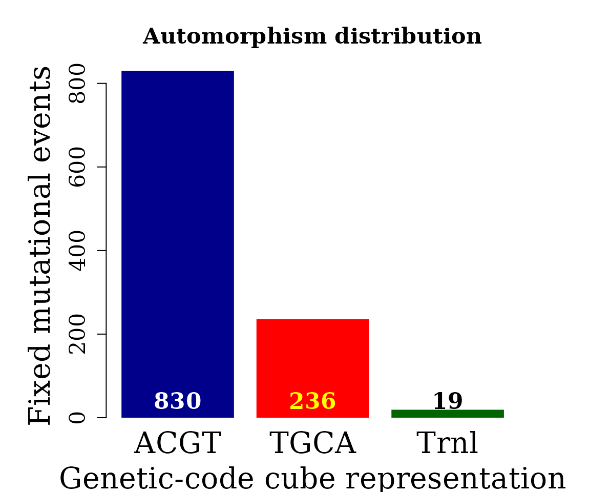
Grouping automorphisms by automorphism coefficients. Types of mutations
autby_coef <- automorphism_bycoef(covid_autm)
autby_coef <- autby_coef[ autby_coef$autm != 1 & autby_coef$autm != -1  ]
Barplot of the frequency of mutation types greater than 2.
post_prob <- automorphism_prob(autby_coef)
counts <-  post_prob$frequency
names(counts) <- post_prob$Codon
counts <- counts[counts > 2]


par(family = "serif", cex.axis = 2, font = 2, las = 1,
    cex.main = 2.2, mar = c(6,2,4,4))
barplot(counts, main="Automorphism distribution per Mutation type",
        col = colorRampPalette(c("red", "yellow", "blue"))(36),
        border = NA, axes = FALSE,las=2)
axis(side = 2,  cex.axis = 2, line = -1.8 )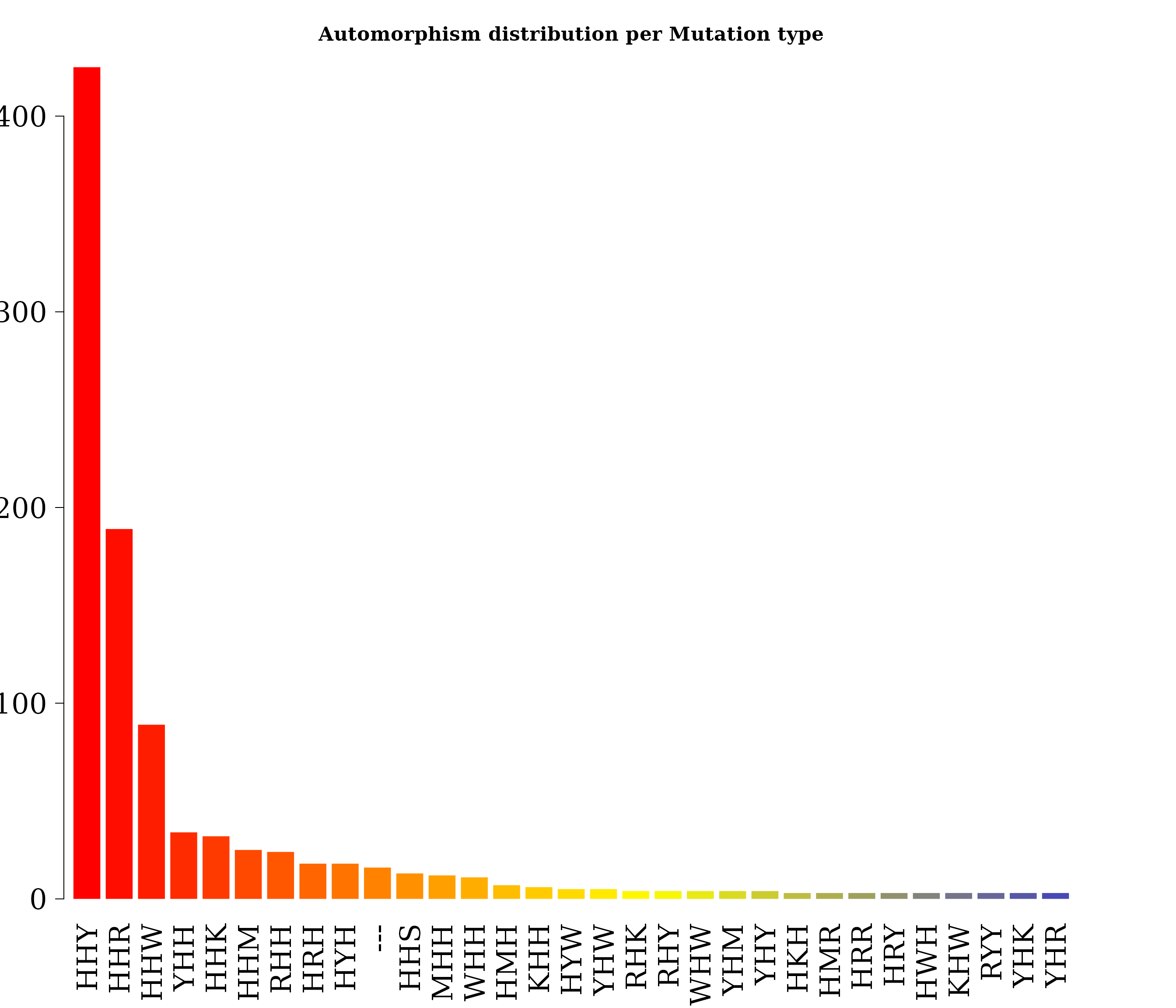
Every single base mutational event across the MSA was classified according to IUPAC nomenclature: 1) According to the number of hydrogen bonds (on DNA/RNA double helix): strong S={C, G} (three hydrogen bonds) and weak W={A, T} (two hydrogen bonds). 2) According to the chemical type: purines R={A, G} and pyrimidines Y={C, T}. 3) According to the presence of amino or keto groups on the base rings: amino M={C, A} and keto K={G, T}. Insertion-deletion mutational events are represented by symbol ‘—’. Constant (hold) base positions were labeled with letter H. So, codon positions labeled as HKH means that the first and third bases remain constant and mutational events between bases G and T were found in the MSA.
We applied a Dirichlet-Multinomial Modelling (in a Bayesian framework) to compute the posterior probability of each type of mutational event, where the posterior Dirichlet distribution is:
where the are known as initial concentration parameters, which represent our initial belief or assumption about the distribution of the mutation types, and stands for the observed frequencies:
post_prob <- post_prob[post_prob$Posterior_Probability > 0.003,]
post_prob
#>    Codon frequency     alpha Posterior_Probability
#> 1    HHY       425 4.1228070           0.363134174
#> 2    HHR       189 4.1228070           0.163425224
#> 3    HHW        89 4.1228070           0.078802788
#> 4    YHH        34 4.0936822           0.032235802
#> 5    HHK        32 3.8804599           0.030362919
#> 6    HHM        25 3.1326061           0.023806497
#> 7    RHH        24 3.0263325           0.022870341
#> 8    HRH        18 2.3866533           0.017251683
#> 9    HYH        18 2.3866533           0.017251683
#> 10   HHS        13 1.8453874           0.012562529
#> 11   MHH        12 1.7374407           0.011624957
#> 12   WHH        11 1.6295573           0.010687439
#> 13   HMH         7 1.1875831           0.006928532
#> 14   KHH         6 1.0742652           0.005986416
#> 15   HYW         5 0.9592506           0.005042863
#> 16   YHW         5 0.9592506           0.005042863
#> 17   RHK         4 0.8407656           0.004096374
#> 18   RHY         4 0.8407656           0.004096374
#> 19   WHW         4 0.8407656           0.004096374
#> 20   YHM         4 0.8407656           0.004096374
#> 21   YHY         4 0.8407656           0.004096374
#> 22   HKH         3 0.7170588           0.003145466
#> 23   HMR         3 0.7170588           0.003145466
#> 24   HRR         3 0.7170588           0.003145466
#> 25   HRY         3 0.7170588           0.003145466
#> 26   HWH         3 0.7170588           0.003145466
#> 27   KHW         3 0.7170588           0.003145466
#> 28   RYY         3 0.7170588           0.003145466
#> 29   YHK         3 0.7170588           0.003145466
#> 30   YHR         3 0.7170588           0.003145466
The analysis of the frequency of mutational events (automorphisms, COVID: human SARS coronavirus GZ02 vs Bat SARS-like coronavirus isolate bat-SL-CoVZC45) by mutation types is shown in the last figure. Results are consistent with the well-known observation highlighted by Crick: the highest mutational rate is found in the third base of the codon (HHY: 425, HHR: 189, HHW: 88), followed by YHH: 34 in the first base, and the lowest rate is found in the second one (5).
probs <- post_prob$Posterior_Probability
names(probs) <- post_prob$Codon

par(family = "serif", cex.axis = 2, font = 2, las = 1,
    cex.main = 2.1, mar = c(7,2,4,2))
barplot(probs, main="Automorphism Probability per Mutation type",
        col = colorRampPalette(c("red", "yellow", "blue"))(36),
        border = NA, axes = FALSE,las = 2, hadj = 0.8)
axis(side = 2,  cex.axis = 2.1, line = -1.8, hadj = 0.9 )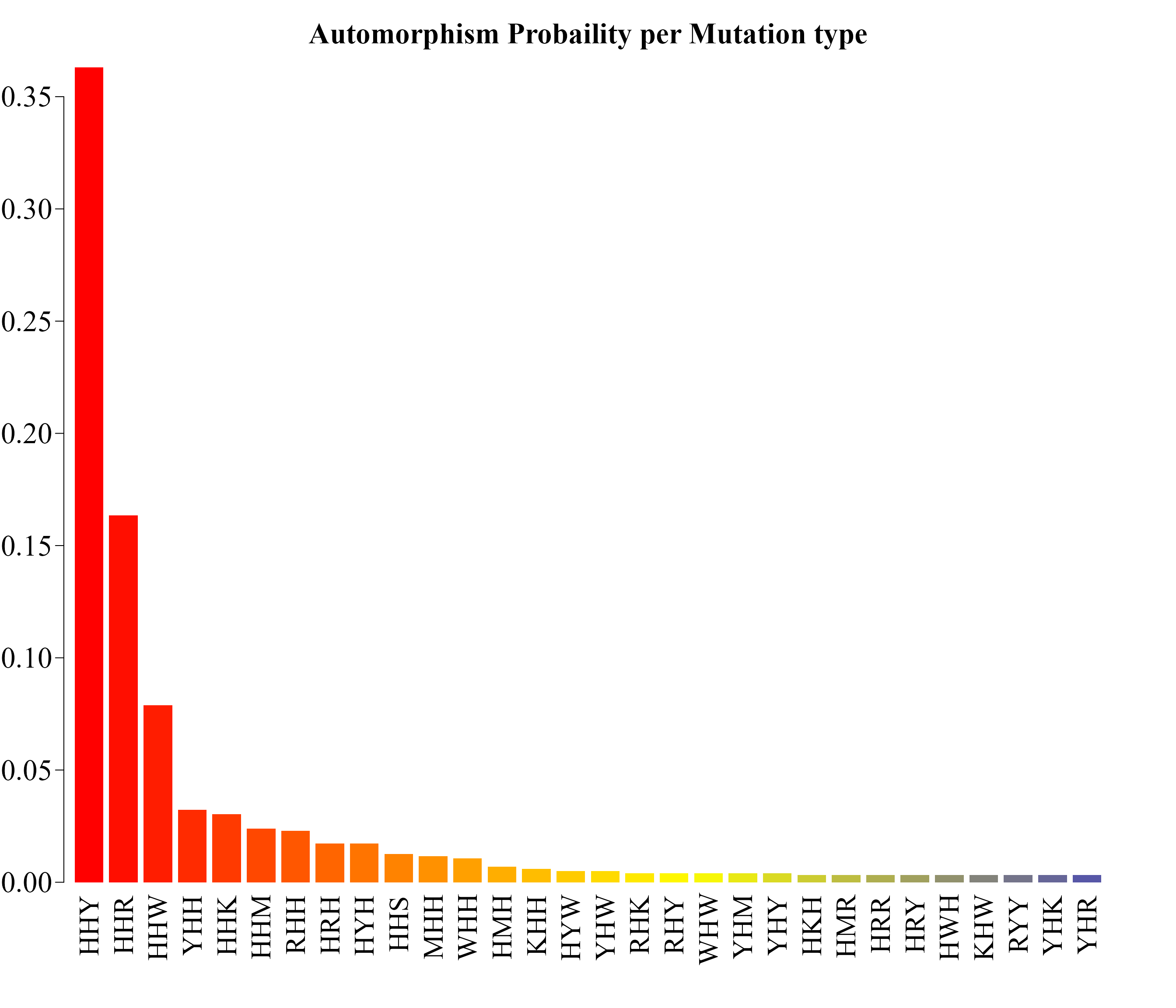
Conserved and non-conserved regions
Conserved regions
Conserved and non-conserved gene regions can be easily observed in most MSA-editing bioinformatic tools. However, here we are interested in obtaining the region coordinates for further downstream analysis.
Conserved regions from pairwise comparisons are obtained with the
conserved_regions function:
conserv <- conserved_regions(covid_autm)
conserv
#> AutomorphismByCoef object with 6348 ranges and 7 metadata columns:
#>          seqnames    ranges strand |        seq1        seq2         aa1         aa2      autm    mut_type        cube
#>             <Rle> <IRanges>  <Rle> | <character> <character> <character> <character> <numeric> <character> <character>
#>      [1]        1      1-19      + |         ATG         ATG           M           M         1         HHH        ACGT
#>      [2]        1      1-19      + |         GAG         GAG           E           E         1         HHH        ACGT
#>      [3]        1      1-19      + |         AGC         AGC           S           S         1         HHH        ACGT
#>      [4]        1      1-19      + |         CTT         CTT           L           L         1         HHH        ACGT
#>      [5]        1      1-19      + |         GTT         GTT           V           V         1         HHH        ACGT
#>      ...      ...       ...    ... .         ...         ...         ...         ...       ...         ...         ...
#>   [6344]        1 9683-9722      + |         GGA         GGA           G           G         1         HHH        ACGT
#>   [6345]        1 9683-9722      + |         TCT         TCT           S           S         1         HHH        ACGT
#>   [6346]        1 9683-9722      + |         TCA         TCA           S           S         1         HHH        ACGT
#>   [6347]        1 9683-9722      + |         GCA         GCA           A           A         1         HHH        ACGT
#>   [6348]        1 9683-9722      + |         TAA         TAA           *           *         1         HHH        ACGT
#>   -------
#>   seqinfo: 1 sequence from an unspecified genome; no seqlengths
Several regions are shared by more than one comparison.
conserv_unique <- conserved_regions(covid_autm, output = "unique")
conserv_unique
#> GRanges object with 744 ranges and 2 metadata columns:
#>         seqnames    ranges strand |      autm        cube
#>            <Rle> <IRanges>  <Rle> | <numeric> <character>
#>     [1]        1      1-19      + |         1        ACGT
#>     [2]        1     21-44      + |         1        ACGT
#>     [3]        1     47-52      + |         1        ACGT
#>     [4]        1     54-60      + |         1        ACGT
#>     [5]        1     62-80      + |         1        ACGT
#>     ...      ...       ...    ... .       ...         ...
#>   [740]        1 9610-9614      + |         1        ACGT
#>   [741]        1 9616-9648      + |         1        ACGT
#>   [742]        1 9650-9674      + |         1        ACGT
#>   [743]        1 9676-9681      + |         1        ACGT
#>   [744]        1 9683-9722      + |         1        ACGT
#>   -------
#>   seqinfo: 1 sequence from an unspecified genome; no seqlengths
Automorphisms on
Alternatively, we can use the algebraic representation on .
autm_z125 <- automorphisms(
                    seqs = covid_aln,
                    group = "Z125",
                    cube = c("ACGT", "TGCA"),
                    cube_alt = c("CATG", "GTAC"),
                    verbose = FALSE)
For the sake of reducing computational time in this example, ‘autm_z125’ is available with the package.
data(autm_z125, package = "GenomAutomorphism")
autm_z125
#> Automorphism object with 9722 ranges and 8 metadata columns:
#>          seqnames    ranges strand |        seq1        seq2         aa1         aa2    coord1    coord2      autm
#>             <Rle> <IRanges>  <Rle> | <character> <character> <character> <character> <numeric> <numeric> <numeric>
#>      [1]        1         1      + |         ATG         ATG           M           M       108       108         1
#>      [2]        1         2      + |         GAG         GAG           E           E        43        43         1
#>      [3]        1         3      + |         AGC         AGC           S           S        82        82         1
#>      [4]        1         4      + |         CTT         CTT           L           L       114       114         1
#>      [5]        1         5      + |         GTT         GTT           V           V       119       119         1
#>      ...      ...       ...    ... .         ...         ...         ...         ...       ...       ...       ...
#>   [9718]        1      9718      + |         TCA         TCA           S           S        71        71         1
#>   [9719]        1      9719      + |         ACT         ACT           T           T        59        59         1
#>   [9720]        1      9720      + |         CAG         CAG           Q           Q        38        38         1
#>   [9721]        1      9721      + |         GCA         GCA           A           A        66        66         1
#>   [9722]        1      9722      + |         TAA         TAA           *           *        46        46         1
#>                 cube
#>          <character>
#>      [1]        ACGT
#>      [2]        ACGT
#>      [3]        ACGT
#>      [4]        ACGT
#>      [5]        ACGT
#>      ...         ...
#>   [9718]        ACGT
#>   [9719]        ACGT
#>   [9720]        ACGT
#>   [9721]        ACGT
#>   [9722]        ACGT
#>   -------
#>   seqinfo: 1 sequence from an unspecified genome; no seqlengths
And the summary by range
aut_range_2 <- automorphismByRanges(autm_z125)
aut_range_2
#> GRanges object with 21 ranges and 1 metadata column:
#>        seqnames    ranges strand |        cube
#>           <Rle> <IRanges>  <Rle> | <character>
#>    [1]        1     1-943      + |        ACGT
#>    [2]        1       944      + |        Trnl
#>    [3]        1   945-970      + |        ACGT
#>    [4]        1       971      + |        Trnl
#>    [5]        1  972-7076      + |        ACGT
#>    ...      ...       ...    ... .         ...
#>   [17]        1 9258-9276      + |        ACGT
#>   [18]        1 9277-9279      + |        Trnl
#>   [19]        1 9280-9294      + |        ACGT
#>   [20]        1 9295-9296      + |        Trnl
#>   [21]        1 9297-9722      + |        ACGT
#>   -------
#>   seqinfo: 1 sequence from an unspecified genome; no seqlengths
The whole genome can be described by automorphisms on .
counts <- table(autm_z125$cube[ autm_z125$autm != 1 ])

par(family = "serif", cex = 1, font = 2)
barplot(counts, main="Automorphism distribution",
        xlab="Genetic-code cube representation",
        ylab="Fixed mutational events",
        col=c("darkblue","red"),
        ylim = c(0, 1300),
        border = NA, axes = TRUE)
mtext(side = 1,line = -2, at = c(0.7, 1.9, 3.1),
    text = paste0( counts ), cex = 1.4,
    col = c("white","red"))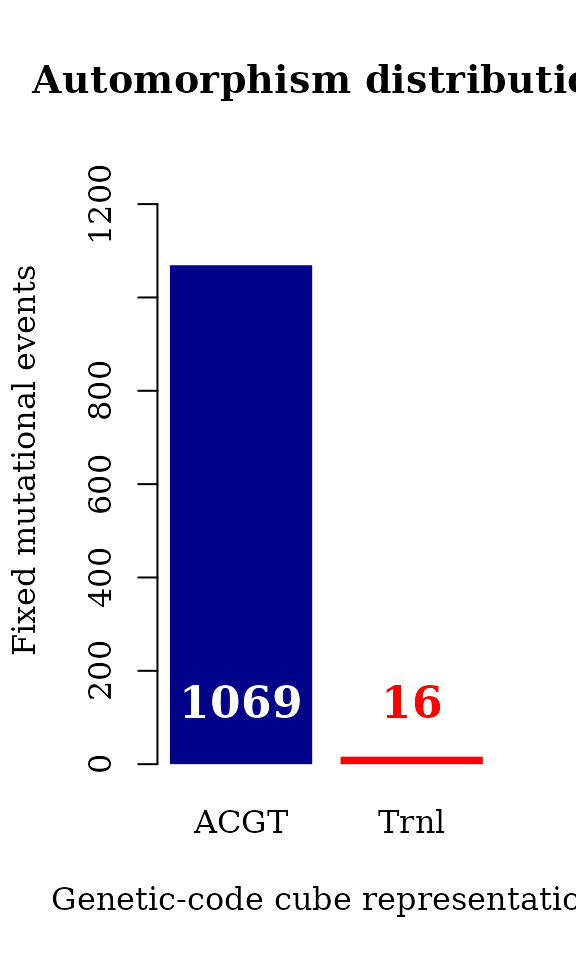
Automorphisms on the Genetic-code Cube Representation on GF(5)
The Genetic-code Cube Representations on the Galois Field GF(5) were studied in (4). Each codon is represented by a coordinate in the 3D space.
Automorphisms are described as functions , where is a diagonal matrix with elements in .
autm_3d <- automorphisms(
                    seqs = covid_aln,
                    group = "Z5^3",
                    cube = c("ACGT", "TGCA"),
                    cube_alt = c("CATG", "GTAC"),
                    verbose = FALSE)
The result is available with the package
data(autm_3d, package = "GenomAutomorphism")
autm_3d
#> Automorphism object with 9722 ranges and 8 metadata columns:
#>          seqnames    ranges strand |        seq1        seq2         aa1         aa2   coord1   coord2        autm
#>             <Rle> <IRanges>  <Rle> | <character> <character> <character> <character> <matrix> <matrix> <character>
#>      [1]        1         1      + |         ATG         ATG           M           M    1:4:3    1:4:3       1,1,1
#>      [2]        1         2      + |         GAG         GAG           E           E    3:1:3    3:1:3       1,1,1
#>      [3]        1         3      + |         AGC         AGC           S           S    1:3:2    1:3:2       1,1,1
#>      [4]        1         4      + |         CTT         CTT           L           L    2:4:4    2:4:4       1,1,1
#>      [5]        1         5      + |         GTT         GTT           V           V    3:4:4    3:4:4       1,1,1
#>      ...      ...       ...    ... .         ...         ...         ...         ...      ...      ...         ...
#>   [9718]        1      9718      + |         TCA         TCA           S           S    4:2:1    4:2:1       1,1,1
#>   [9719]        1      9719      + |         ACT         ACT           T           T    1:2:4    1:2:4       1,1,1
#>   [9720]        1      9720      + |         CAG         CAG           Q           Q    2:1:3    2:1:3       1,1,1
#>   [9721]        1      9721      + |         GCA         GCA           A           A    3:2:1    3:2:1       1,1,1
#>   [9722]        1      9722      + |         TAA         TAA           *           *    4:1:1    4:1:1       1,1,1
#>                 cube
#>          <character>
#>      [1]        ACGT
#>      [2]        ACGT
#>      [3]        ACGT
#>      [4]        ACGT
#>      [5]        ACGT
#>      ...         ...
#>   [9718]        ACGT
#>   [9719]        ACGT
#>   [9720]        ACGT
#>   [9721]        ACGT
#>   [9722]        ACGT
#>   -------
#>   seqinfo: 1 sequence from an unspecified genome; no seqlengths
Grouping automorphisms by automorphism coefficients
Automorphisms that preserve codons (DNA base-triplets) are represented by the identity matrix, i.e., the matrix with diagonal elements “1,1,1”.
autby_coef_3d <- automorphism_bycoef(autm_3d)
autby_coef_3d <- autby_coef_3d[ autby_coef_3d$autm != "1,1,1" ]
autby_coef_3d
#> AutomorphismByCoef object with 1083 ranges and 7 metadata columns:
#>          seqnames    ranges strand |        seq1        seq2         aa1         aa2        autm    mut_type
#>             <Rle> <IRanges>  <Rle> | <character> <character> <character> <character> <character> <character>
#>      [1]        1        20      + |         GTC         GTT           V           V       1,1,2         HHY
#>      [2]        1     45-46      + |         CAC         CAT           H           H       1,1,2         HHY
#>      [3]        1     45-46      + |         CTC         CTT           L           L       1,1,2         HHY
#>      [4]        1        53      + |         CTA         TTA           L           L       2,1,1         YHH
#>      [5]        1        61      + |         CTG         TTG           L           L       2,1,1         YHH
#>      ...      ...       ...    ... .         ...         ...         ...         ...         ...         ...
#>   [1079]        1      9609      + |         CCA         CCG           P           P       1,1,3         HHR
#>   [1080]        1      9615      + |         TTT         TTC           F           F       1,1,3         HHY
#>   [1081]        1      9649      + |         AAC         AGC           N           S       1,3,1         HRH
#>   [1082]        1      9675      + |         AAA         AAG           K           K       1,1,3         HHR
#>   [1083]        1      9682      + |         TTG         TTA           L           L       1,1,2         HHR
#>                 cube
#>          <character>
#>      [1]        ACGT
#>      [2]        ACGT
#>      [3]        ACGT
#>      [4]        ACGT
#>      [5]        ACGT
#>      ...         ...
#>   [1079]        ACGT
#>   [1080]        ACGT
#>   [1081]        ACGT
#>   [1082]        ACGT
#>   [1083]        ACGT
#>   -------
#>   seqinfo: 1 sequence from an unspecified genome; no seqlengths
Conserved regions from pairwise comparisons are obtained with the
conserved_regions function:
conserv <- conserved_regions(autm_3d)
conserv
#> AutomorphismByCoef object with 6348 ranges and 7 metadata columns:
#>          seqnames    ranges strand |        seq1        seq2         aa1         aa2        autm    mut_type
#>             <Rle> <IRanges>  <Rle> | <character> <character> <character> <character> <character> <character>
#>      [1]        1      1-19      + |         ATG         ATG           M           M       1,1,1         HHH
#>      [2]        1      1-19      + |         GAG         GAG           E           E       1,1,1         HHH
#>      [3]        1      1-19      + |         AGC         AGC           S           S       1,1,1         HHH
#>      [4]        1      1-19      + |         CTT         CTT           L           L       1,1,1         HHH
#>      [5]        1      1-19      + |         GTT         GTT           V           V       1,1,1         HHH
#>      ...      ...       ...    ... .         ...         ...         ...         ...         ...         ...
#>   [6344]        1 9683-9722      + |         GGA         GGA           G           G       1,1,1         HHH
#>   [6345]        1 9683-9722      + |         TCT         TCT           S           S       1,1,1         HHH
#>   [6346]        1 9683-9722      + |         TCA         TCA           S           S       1,1,1         HHH
#>   [6347]        1 9683-9722      + |         GCA         GCA           A           A       1,1,1         HHH
#>   [6348]        1 9683-9722      + |         TAA         TAA           *           *       1,1,1         HHH
#>                 cube
#>          <character>
#>      [1]        ACGT
#>      [2]        ACGT
#>      [3]        ACGT
#>      [4]        ACGT
#>      [5]        ACGT
#>      ...         ...
#>   [6344]        ACGT
#>   [6345]        ACGT
#>   [6346]        ACGT
#>   [6347]        ACGT
#>   [6348]        ACGT
#>   -------
#>   seqinfo: 1 sequence from an unspecified genome; no seqlengths
The whole-genome mutational events are represented as automorphisms on the 3D space , specifically on the cube ACGT (see 4).
counts <- table(autby_coef_3d$cube[ autby_coef_3d$autm != "1,1,1"])

par(family = "serif", cex = 1, font = 2, cex.main = 1)
barplot(counts, main="Automorphism distribution",
        xlab="Genetic-code cube representation",
        ylab="Fixed mutational events",
        col=c("darkblue","red"),
        ylim = c(0, 1300),
        border = NA, axes = TRUE)
mtext(side = 1,line = -2, at = c(0.7, 1.9),
    text = paste0( counts ), cex = 1.4,
    col = c("white"))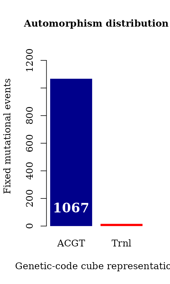
References
1. R. Sanchez. Symmetric Group of the Genetic-Code Cubes.
Effect of the Genetic-Code Architecture on the Evolutionary Process. MATCH
Commun. Math. Comput. Chem. 79 (2018) 527-560.
[PDF](https://bit.ly/2Z9mjM7).

2. Sanchez R, Morgado E, Grau R. Gene algebra from a
genetic code algebraic structure. J Math Biol. 2005 Oct;51(4):431-57.
doi:10.1007/s00285-005-0332-8. Epub 2005 Jul 13. PMID: 16012800.
([PDF](https://arxiv.org/pdf/q-bio/0412033.pdf)).

3. Robersy Sanchez, Jesus Barreto (2021) Genomic Abelian
Finite Groups.
[doi:10.1101/2021.06.01.446543](https://doi.org/10.1101/2021.06.01.446543)

4. M. V. Jose, E.R. Morgado, R. Sanchez, T. Govezensky,
The 24 possible algebraic representations of the standard genetic code in
six or in three dimensions, Adv. Stud. Biol. 4 (2012) 119-152.
[PDF](https://is.gd/na9eap).

5. Crick FHC. The Origin of the Genetic Code. J Mol Biol.
1968;38: 367–379.
Session info
Here is the output of sessionInfo() on the system on
which this document was compiled:
#> R version 4.6.1 (2026-06-24)
#> Platform: x86_64-pc-linux-gnu
#> Running under: Ubuntu 24.04.4 LTS
#>
#> Matrix products: default
#> BLAS:   /usr/lib/x86_64-linux-gnu/blas/libblas.so.3.12.0
#> LAPACK: /usr/lib/x86_64-linux-gnu/lapack/liblapack.so.3.12.0  LAPACK version 3.12.0
#>
#> locale:
#>  [1] LC_CTYPE=C.UTF-8       LC_NUMERIC=C           LC_TIME=C.UTF-8        LC_COLLATE=C.UTF-8     LC_MONETARY=C.UTF-8
#>  [6] LC_MESSAGES=C.UTF-8    LC_PAPER=C.UTF-8       LC_NAME=C              LC_ADDRESS=C           LC_TELEPHONE=C
#> [11] LC_MEASUREMENT=C.UTF-8 LC_IDENTIFICATION=C
#>
#> time zone: America/Chicago
#> tzcode source: system (glibc)
#>
#> attached base packages:
#> [1] stats4    stats     graphics  grDevices utils     datasets  methods   base
#>
#> other attached packages:
#> [1] GenomAutomorphism_1.15.1 Biostrings_2.80.1        Seqinfo_1.2.0            XVector_0.52.0
#> [5] IRanges_2.46.0           S4Vectors_0.50.1         BiocGenerics_0.58.1      generics_0.1.4
#> [9] BiocStyle_2.40.0
#>
#> loaded via a namespace (and not attached):
#>  [1] sass_0.4.10          numbers_0.9-2        digest_0.6.39        magrittr_2.0.5       evaluate_1.0.5
#>  [6] bookdown_0.47        iterators_1.0.14     fastmap_1.2.0        foreach_1.5.2        doParallel_1.0.17
#> [11] jsonlite_2.0.0       BiocManager_1.30.27  codetools_0.2-20     textshaping_1.0.5    jquerylib_0.1.4
#> [16] cli_3.6.6            rlang_1.3.0          crayon_1.5.3         cachem_1.1.0         yaml_2.3.12
#> [21] otel_0.2.0           tools_4.6.1          parallel_4.6.1       BiocParallel_1.46.0  dplyr_1.2.1
#> [26] vctrs_0.7.3          R6_2.6.1             matrixStats_1.5.0    lifecycle_1.0.5      fs_2.1.0
#> [31] htmlwidgets_1.6.4    ragg_1.5.2           pkgconfig_2.0.3      desc_1.4.3           pkgdown_2.2.1
#> [36] bslib_0.11.0         pillar_1.11.1        data.table_1.18.4    glue_1.8.1           systemfonts_1.3.2
#> [41] xfun_0.60            tibble_3.3.1         GenomicRanges_1.64.0 tidyselect_1.2.1     knitr_1.51
#> [46] htmltools_0.5.9      rmarkdown_2.31       compiler_4.6.1