Analysis of Automorphisms on a DNA Multiple Sequence Alignment
Robersy Sanchez
Department of Biology. Pennsylvania State University, University Park, PA 16802rus547@psu.edu
28 December 2024
Source:vignettes/automorphism_on_msa.Rmd
automorphism_on_msa.RmdAbstract
Analysis of DNA mutational events on DNA Multiple Sequence Alignment (MSA) by means of automorphisms between pairwise DNA sequences algebraically represented as Abelian finite group. Herein, show a simple example on how the package can be applied.
Overview
This is a R package to compute the autimorphisms between pairwise aligned DNA sequences represented as elements from a Genomic Abelian group as described in reference (1). In a general scenario, whole chromosomes or genomic regions from a population (from any species or close related species) can be algebraically represented as a direct sum of cyclic groups or more specifically Abelian p-groups. Basically, we propose the representation of multiple sequence alignments (MSA) of length N as a finite Abelian group created by the direct sum of homocyclic Abelian groups of prime-power order:
Where, the ’s are prime numbers, and is the group of integer modulo .
For the purpose of estimating the automorphism between two aligned DNA sequences, .
Automorphisms
Herein, automorphisms are considered algebraic descriptions of mutational event observed in codon sequences represented on different Abelian groups. In particular, as described in references (3-4), for each representation of the codon set on a defined Abelian group there are 24 possible isomorphic Abelian groups. These Abelian groups can be labeled based on the DNA base-order used to generate them. The set of 24 Abelian groups can be described as a group isomorphic to the symmetric group of degree four (, see reference (4)).
For further support about the symmetric group on the 24 Abelian group of genetic-code cubes, users can also see Symmetric Group of the Genetic-Code Cubes., specifically the Mathematica notebook IntroductionToZ5GeneticCodeVectorSpace.nb and interact with it using Wolfram Player, freely available (for Windows and Linux OS) at, https://www.wolfram.com/player/.
Automorphisms on
First, we proceed to load the R package required for our analysis
Next, we proceed to check the DNA multiple sequence alignment (MSA) file. This ia a FASTA file carrying the MSA of mammals (somatic) Cystocrome c. Notice that we are familiar with the FASTA file, then it is better to directly read it with function automorphisms.
However, for the current example, this step can be bypassed, since the MSA is provided provided together with GenomAutomorphism R package
## Do not run it. This is included with package
URL <- paste0("https://github.com/genomaths/seqalignments/raw/master/CYCS/",
              "primate_cytochrome_c_(CYCS)_18_sequences.fasta")

cyc_aln <- readDNAMultipleAlignment(filepath = URL)
Load MSA available in the package
data("cyc_aln")
cyc_aln
#> DNAMultipleAlignment with 19 rows and 318 columns
#>       aln                                                                                           names
#>  [1] ATGGGTGATGTTGAGAAAGGCAAGAAGATTTTTATTATGAAGTGT...AGGGCAGACTTAATAGCTTATCTCAAAAAAGCTACTAATGAGTAA NM_018947.6 Homo ...
#>  [2] ATGGGTGATGTTGAGAAAGGCAAGAAGATTTTTATTATGAAGTGT...AGGGCAGACTTAATAGCTTATCTCAAAAAAGCTACTAATGAGTAA gb|BC021994.1|  [...
#>  [3] ATGGGTGATGTTGAGAAAGGCAAGAAGATTTTTATTATGAAGTGT...AGGGCAGACTTAATAGCTTATCTCAAAAAAGCTACTAATGAGTAA ref|XM_019031021....
#>  [4] ATGGGTGATGTTGAGAAAGGCAAGAAGATTTTTATTATGAAGTGT...AGGGCAGACTTAATAGCTTATCTCAAAAAAGCTACTAATGAGTAA dbj|AK311836.1|  ...
#>  [5] ATGGGTGATGTTGAGAAAGGCAAGAAGATTTTTATTATGAAGTGT...AGGGCAGACTTAATAGCTTATCTCAAAAAAGCTACTAATGAGTAA gb|BC067222.1|  [...
#>  [6] ATGGGTGATGTTGAGAAAGGCAAGAAGATTTTTATTATGAAGTGT...AGGGCAGACTTAATAGCTTATCTCAAAAAAGCTACTAATGAGTAA gb|BC068464.1|  [...
#>  [7] ATGGGTGATGTTGAGAAAGGCAAGAAGATTTTTATTATGAAGTGT...AGGGCAGACTTAATAGCTTATCTCAAAAAAGCTACTAATGAGTAA gb|BC015130.1|  [...
#>  [8] ATGGGTGATGTTGAGAAAGGCAAGAAGATTTTTATTATGAAGTGT...AGGGCAGACTTGATAGCTTATCTCAAAAAAGCTACTAATGAGTAA ref|XM_032759077....
#>  [9] ATGGGTGATGTTGAGAAAGGCAAGAAGATTTTTATTATGAAGTGT...AGGGCAGACTTGATAGCTTATCTCAAAAAAGCTACTAATGAGTAA ref|XM_003270423....
#> [10] ATGGGTGATGTTGAGAAAGGCAAGAAGATTTTTATTATGAAGTGT...AGGGCAGACTTGATAGCTTATCTCAAAAAAGCTACTAATGAGTAA ref|XM_033192823....
#> [11] ATGGGTGATGTTGAGAAAGGCAAGAAGATTTTTATTATGAAGTGT...AGGGCAGACTTGATAGCTTATCTCAAAAAAGCTACTAATGAGTAA ref|XM_003896182....
#> [12] ATGGGTGATGTTGAGAAAGGCAAGAAGATTTTTATTATGAAGTGT...AGGGCAGACTTGATAGCTTATCTCAAAAAAGCTACTAATGAGTAA ref|XM_003895240....
#> [13] ATGGGTGATGTTGAGAAAGGCAAGAAGATTTTTATTATGAAGTGT...AGGGCAGACTTGATAGCTTATCTCAAAAAAGCTACTAATGAGTAA ref|XM_010375926....
#> [14] ATGGGTGATGTTGAGAAAGGCAAGAAGATTTTTATTATGAAGTGT...AGGGCAGACTTGATAGCTTATCTCAAAAAAGCTACTAATGAGTAA ref|XM_028845949....
#> [15] ATGGGTGATGTTGAGAAAGGCAAGAAGATTTTTATTATGAAGTGT...AGGGCAGACTTGATAGCTTATCTCAAAAAAGCTACTAATGAGTAA ref|XM_028845948....
#> [16] ATGGGTGATGTTGAGAAAGGCAAGAAGATTTTTATTATGAAGTGT...AGGGCAGACTTGATAGCTTATCTCAAAAAAGCTACTAATGAGTAA ref|XM_025380676....
#> [17] ATGGGTGATGTTGAGAAAGGCAAGAAGATTTTTATTATGAAGTGT...AGGGCAGACTTGATAGCTTATCTCAAAAAAGCTACTAATGAGTAA ref|XM_025380675....
#> [18] ATGGGTGATGTTGAGAAAGGCAAGAAGATTTTTATTATGAAGTGT...AGGGCAGACTTAATAGCTTATCTCAAAAAAGCTACTAATGAGTAA ref|NM_001131167....
#> [19] ATGGGTGATGTTGAGAAAGGCAAGAAGATTTTTATTATGAAGTGT...AGGGCAGACTTAATAGCTTATCTCAAAAAAGCTACTAATGAGTAA emb|CR857183.1|  ...
The sequence names
strtrim(rownames(cyc_aln), 100)
#>  [1] "NM_018947.6 Homo sapiens cytochrome c, somatic (CYCS), mRNA"
#>  [2] "gb|BC021994.1|  [organism=Homo sapiens] [note=Vector: pDNR-LIB] [gcode=1] [clone=MGC:24510 IMAGE:409"
#>  [3] "ref|XM_019031021.2|  [location=chromosome] [chromosome=7] [organism=Gorilla gorilla gorilla] [isolat"
#>  [4] "dbj|AK311836.1|  [organism=Homo sapiens] [gcode=1] [clone=BRACE3022676] [tissue_type=cerebellum] [cl"
#>  [5] "gb|BC067222.1|  [organism=Homo sapiens] [note=Vector: pDNR-LIB] [gcode=1] [clone=MGC:72005 IMAGE:368"
#>  [6] "gb|BC068464.1|  [organism=Homo sapiens] [note=Vector: pBluescriptR] [gcode=1] [clone=MGC:87065 IMAGE"
#>  [7] "gb|BC015130.1|  [organism=Homo sapiens] [note=Vector: pDNR-LIB] [gcode=1] [clone=MGC:24248 IMAGE:393"
#>  [8] "ref|XM_032759077.1|  [chromosome=Unknown] [organism=Hylobates moloch] [isolate=HMO894] [note=Lionel]"
#>  [9] "ref|XM_003270423.4|  [location=chromosome] [chromosome=17] [organism=Nomascus leucogenys] [isolate=A"
#> [10] "ref|XM_033192823.1|  [chromosome=Unknown] [organism=Trachypithecus francoisi] [isolate=TF-2019V2] [g"
#> [11] "ref|XM_003896182.3|  [location=chromosome] [chromosome=4] [organism=Papio anubis] [isolate=15944] [g"
#> [12] "ref|XM_003895240.5|  [location=chromosome] [chromosome=2] [organism=Papio anubis] [isolate=15944] [g"
#> [13] "ref|XM_010375926.2|  [location=chromosome] [chromosome=6] [organism=Rhinopithecus roxellana] [isolat"
#> [14] "ref|XM_028845949.1|  [location=chromosome] [chromosome=3] [organism=Macaca mulatta] [isolate=AG07107"
#> [15] "ref|XM_028845948.1|  [location=chromosome] [chromosome=3] [organism=Macaca mulatta] [isolate=AG07107"
#> [16] "ref|XM_025380676.1|  [location=chromosome] [chromosome=3] [organism=Theropithecus gelada] [isolate=D"
#> [17] "ref|XM_025380675.1|  [location=chromosome] [chromosome=3] [organism=Theropithecus gelada] [isolate=D"
#> [18] "ref|NM_001131167.2|  [chromosome=7] [organism=Pongo abelii] [gcode=1] [chromosome=7] [map=7] Pongo a"
#> [19] "emb|CR857183.1|  [organism=Pongo abelii] [gcode=1] [clone=DKFZp468F1016] [tissue_type=heart] [clone_"
The corresponding aminoacid sequence is:
translate(cyc_aln@unmasked)
#> AAStringSet object of length 19:
#>      width seq                                                                                      names
#>  [1]   106 MGDVEKGKKIFIMKCSQCHTVEKGGKHKTGPNLHGLFGRKTGQ...LMEYLENPKKYIPGTKMIFVGIKKKEERADLIAYLKKATNE* NM_018947.6 Homo ...
#>  [2]   106 MGDVEKGKKIFIMKCSQCHTVEKGGKHKTGPNLHGLFGRKTGQ...LMEYLENPKKYIPGTKMIFVGIKKKEERADLIAYLKKATNE* gb|BC021994.1|  [...
#>  [3]   106 MGDVEKGKKIFIMKCSQCHTVEKGGKHKTGPNLHGLFGRKTGQ...LMEYLENPKKYIPGTKMIFVGIKKKEERADLIAYLKKATNE* ref|XM_019031021....
#>  [4]   106 MGDVEKGKKIFIMKCSQCHTVEKGGKHKTGPNLHGLFGRKTGQ...LMEYLENPKKYIPGTKMIFVGIKKKEERADLIAYLKKATNE* dbj|AK311836.1|  ...
#>  [5]   106 MGDVEKGKKIFIMKCSQCHTVEKGGKHKTGPNLHGLFGRKTGQ...LMEYLENPKKYIPGTKMIFVGIKKKEERADLIAYLKKATNE* gb|BC067222.1|  [...
#>  ...   ... ...
#> [15]   106 MGDVEKGKKIFIMKCSQCHTVEKGGKHKTGPNLHGLFGRKTGQ...LMEYLENPKKYIPGTKMIFVGIKKKEERADLIAYLKKATNE* ref|XM_028845948....
#> [16]   106 MGDVEKGKKIFIMKCSQCHTVEKGGKHKTGPNLHGLFGRKTGQ...LMEYLENPKKYIPGTKMIFVGIKKKEERADLIAYLKKATNE* ref|XM_025380676....
#> [17]   106 MGDVEKGKKIFIMKCSQCHTVEKGGKHKTGPNLHGLFGRKTGQ...LMEYLENPKKYIPGTKMIFVGIKKKEERADLIAYLKKATNE* ref|XM_025380675....
#> [18]   106 MGDVEKGKKIFIMKCSQCHTVEKGGKHKTGPNLHGLFGRKTGQ...LMEYLENPKKYIPGTKMIFVGIKKKEERADLIAYLKKATNE* ref|NM_001131167....
#> [19]   106 MGDVEKGKKIFIMKCSQCHTVEKGGKHKTGPNLHGLFGRKTGQ...LMEYLENPKKYIPGTKMIFVGIKKKEERADLIAYLKKATNE* emb|CR857183.1|  ...
Next, function automorphisms will be applied to represent the codon sequence in the Abelian group (i.e., the set of integers remainder modulo 64). The codon coordinates are requested on the cube ACGT. Following reference (4)), cubes are labeled based on the order of DNA bases used to define the sum operation.
In Z64, automorphisms are described as functions , where and are elements from the set of integers modulo 64. Below, in function automorphisms three important arguments are given values: group = “Z64”, cube = c(“ACGT”, “TGCA”), and cube_alt = c(“CATG”, “GTAC”). Setting for group specifies on which group the automorphisms will be computed. These groups can be: “Z5”, “Z64”, “Z125”, and “Z5^3”.
In groups “Z64” and “Z125” not all the mutational events can be described as automorphisms from a given cube. So, a character string denoting pairs of “dual” the genetic-code cubes, as given in references (1-4)), is given as argument for cube. That is, the base pairs from the given cubes must be complementary each other. Such a cube pair are call dual cubes and, as shown in reference (4)), each pair integrates group. If automorphisms are not found in first set of dual cubes, then the algorithm search for automorphism in a alternative set of dual cubes.
## Do not run it. This is included with package

nams <- c("human_1", "human_2", "gorilla", "human_3", "human_4",
          "human_5", "human_6", "silvery_gibbon", "white_cheeked_gibbon",
          "françois_langur", "olive_baboon_1", "olive_baboon_2",
          "golden_monkey", "rhesus_monkeys_1", "rhesus_monkeys_2",
          "gelada_baboon_1", "gelada_baboon_2", "orangutan_1", "orangutan_2")

cyc_autm <- automorphisms(filepath = URL,
                      group = "Z64",
                      cube = c("ACGT", "TGCA"),
                      cube_alt = c("CATG", "GTAC"),
                      nms = nams,
                      verbose = FALSE)
Object autm is included with package and can be load typing:
data(cyc_autm, package = "GenomAutomorphism")
cyc_autm
#> AutomorphismList object of length: 171
#> names(171): human_1.human_2 human_1.gorilla human_1.human_3 ... gelada_baboon_2.orangutan_1 gelada_baboon_2.orangutan_2 orangutan_1.orangutan_2
#> -------
#> Automorphism object with 106 ranges and 8 metadata columns:
#>         seqnames    ranges strand |        seq1        seq2         aa1         aa2    coord1    coord2      autm
#>            <Rle> <IRanges>  <Rle> | <character> <character> <character> <character> <numeric> <numeric> <numeric>
#>     [1]        1         1      + |         ATG         ATG           M           M        50        50         1
#>     [2]        1         2      + |         GGT         GGT           G           G        43        43         1
#>     [3]        1         3      + |         GAT         GAT           D           D        11        11         1
#>     [4]        1         4      + |         GTT         GTT           V           V        59        59         1
#>     [5]        1         5      + |         GAG         GAG           E           E        10        10         1
#>     ...      ...       ...    ... .         ...         ...         ...         ...       ...       ...       ...
#>   [102]        1       102      + |         GCT         GCT           A           A        27        27         1
#>   [103]        1       103      + |         ACT         ACT           T           T        19        19         1
#>   [104]        1       104      + |         AAT         AAT           N           N         3         3         1
#>   [105]        1       105      + |         GAG         GAG           E           E        10        10         1
#>   [106]        1       106      + |         TAA         TAA           *           *        12        12         1
#>                cube
#>         <character>
#>     [1]        ACGT
#>     [2]        ACGT
#>     [3]        ACGT
#>     [4]        ACGT
#>     [5]        ACGT
#>     ...         ...
#>   [102]        ACGT
#>   [103]        ACGT
#>   [104]        ACGT
#>   [105]        ACGT
#>   [106]        ACGT
#>   -------
#>   seqinfo: 1 sequence from an unspecified genome; no seqlengths
#> ...
#> <170 more DFrame element(s)>
#> Two slots: 'DataList' & 'SeqRanges'
#> -------
An AutomorphismList class object is returned. The codon sequences (seq1 and seq2) with their corresponding coordinates (left) are returned, as well as the coordinated representation on (coord1 and coord2). Observe that two new columns were added, the automorphism coefficient (named as autm) and the genetic-code cube where the automorphism was found. By convention the DNA sequence is given for the positive strand. Since the dual cube of “ACGT” corresponds to the complementary base order TGCA, automorphisms described by the cube TGCA represent mutational events affecting the DNA negative strand (-).
Bar plot automorphism distribution by cubes
The automorphism distribution by cubes can be summarized in the bar-plot graphic
counts <- table(unlist(lapply(cyc_autm@DataList,
            function(x) {
              x = data.frame(x)
              x =  x[ x$autm != 1 | is.na(x$autm), ]
              return(x$cube)}
            )
        ))

par(family = "serif", cex = 0.8, font = 2, mar = c(4,6,4,4))
barplot(counts, #main="Automorphism distribution",
        xlab="Genetic-code cube representation",
        ylab="Fixed mutational events",
col=c("darkblue","red", "darkgreen", "magenta", "orange"),
        border = NA, axes = FALSE, ylim = c(0,300),
        cex.lab = 2, cex.main = 1.5, cex.names = 2)
axis(2, at = c(0, 100, 200, 300), cex.axis = 1.5)
mtext(side = 1,line = -1.5, at = c(0.7, 1.9),
      text = paste0( counts ), cex = 1.4,
      col = c("white","yellow"))
Bar plot automorphism distribution by regions
The last result can be summarized by gene regions as follow:
autm_range <- automorphismByRanges(cyc_autm,
                                  min.len = 2,
                                  verbose = FALSE)
autm_range
#> GRangesList object of length 108:
#> $human_1.human_4
#> GRanges object with 3 ranges and 1 metadata column:
#>       seqnames    ranges strand |        cube
#>          <Rle> <IRanges>  <Rle> | <character>
#>   [1]        1      1-60      + |        ACGT
#>   [2]        1        61      + |        TGCA
#>   [3]        1    62-106      + |        ACGT
#>   -------
#>   seqinfo: 1 sequence from an unspecified genome; no seqlengths
#>
#> $human_1.silvery_gibbon
#> GRanges object with 3 ranges and 1 metadata column:
#>       seqnames    ranges strand |        cube
#>          <Rle> <IRanges>  <Rle> | <character>
#>   [1]        1      1-94      + |        ACGT
#>   [2]        1        95      + |        TGCA
#>   [3]        1    96-106      + |        ACGT
#>   -------
#>   seqinfo: 1 sequence from an unspecified genome; no seqlengths
#>
#> $human_1.white_cheeked_gibbon
#> GRanges object with 3 ranges and 1 metadata column:
#>       seqnames    ranges strand |        cube
#>          <Rle> <IRanges>  <Rle> | <character>
#>   [1]        1      1-94      + |        ACGT
#>   [2]        1        95      + |        TGCA
#>   [3]        1    96-106      + |        ACGT
#>   -------
#>   seqinfo: 1 sequence from an unspecified genome; no seqlengths
#>
#> ...
#> <105 more elements>
That is, function automorphismByRanges permits the classification of the pairwise alignment of protein-coding sub-regions based on the mutational events observed on it quantitatively represented as automorphisms on genetic-code cubes.
Searching for automorphisms on permits us a quantitative differentiation between mutational events at different codon positions from a given DNA protein-encoding region. As shown in reference (4)) a set of different cubes can be applied to describe the best evolutionary aminoacid scale highly correlated with aminoacid physicochemical properties describing the observed evolutionary process in a given protein.
More information about this subject can be found in the supporting material from reference (4)) at GitHub GenomeAlgebra_SymmetricGroup, particularly by interacting with the Mathematica notebook Genetic-Code-Scales_of_Amino-Acids.nb.
The automorphism distribution by cubes can be summarized in the bar-plot graphic
cts <- unlist(autm_range)
counts <- table(cts$cube)

par(family = "serif", cex = 0.6, font = 2, las = 1)
barplot(counts, main="Automorphism distribution",
        xlab="Genetic-code cube representation",
        col=c("darkblue","red", "darkgreen"),
        border = NA, axes = T)
mtext(side = 1,line = -6, at = c(0.7, 1.9, 3.1),
      text = paste0( counts ), cex = 1.4,
      col = c("white","yellow"))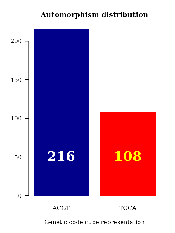
Grouping automorphism by automorphism’s coefficients
Automorphisms with the same automorphism’s coefficients can be grouped.
autby_coef <- automorphism_bycoef(cyc_autm,
                                 verbose = FALSE)
autby_coef
#> AutomorphismByCoefList object of length 171:
#> $human_1.human_2
#> AutomorphismByCoef object with 45 ranges and 7 metadata columns:
#>        seqnames    ranges strand |        seq1        seq2         aa1         aa2      autm    mut_type        cube
#>           <Rle> <IRanges>  <Rle> | <character> <character> <character> <character> <numeric> <character> <character>
#>    [1]        1     1-106      + |         ATG         ATG           M           M         1         HHH        ACGT
#>    [2]        1     1-106      + |         GGT         GGT           G           G         1         HHH        ACGT
#>    [3]        1     1-106      + |         GAT         GAT           D           D         1         HHH        ACGT
#>    [4]        1     1-106      + |         GTT         GTT           V           V         1         HHH        ACGT
#>    [5]        1     1-106      + |         GAG         GAG           E           E         1         HHH        ACGT
#>    ...      ...       ...    ... .         ...         ...         ...         ...       ...         ...         ...
#>   [41]        1     1-106      + |         GAC         GAC           D           D         1         HHH        ACGT
#>   [42]        1     1-106      + |         TTA         TTA           L           L         1         HHH        ACGT
#>   [43]        1     1-106      + |         ATA         ATA           I           I         1         HHH        ACGT
#>   [44]        1     1-106      + |         GCT         GCT           A           A         1         HHH        ACGT
#>   [45]        1     1-106      + |         TAA         TAA           *           *         1         HHH        ACGT
#>   -------
#>   seqinfo: 1 sequence from an unspecified genome; no seqlengths
#>
#> ...
#> <170 more elements>
Every single base mutational event across the MSA was classified according IUPAC nomenclature: 1) According to the number of hydrogen bonds (on DNA/RNA double helix): strong S={C, G} (three hydrogen bonds) and weak W={A, U} (two hydrogen bonds). According to the chemical type: purines R={A, G} and pyrimidines Y={C, U}. 3). According to the presence of amino or keto groups on the base rings: amino M={C, A} and keto K={G, T}. Constant (hold) base positions were labeled with letter H. So, codon positions labeled as HKH means that the first and third bases remains constant and mutational events between bases G and T were found in the MSA.
cts <- unlist(autby_coef)
counts <- table(cts$mut_type[ cts$autm != 1 & cts$autm != -1 ])
counts <- sort(counts, decreasing = TRUE)

par(family = "serif", cex.axis = 1.4, font = 2, las = 1,
    cex.main = 1.4, cex.lab = 2)
barplot(counts, main="Automorphism distribution per Mutation type",
        col = c("red", "orange", "yellow", "green", "dodgerblue"),
        border = NA, axes = TRUE,las=2)
mtext(side = 1,line = -2, at = c(0.7, 1.9, 3.1, 4.3, 5.5),
      text = paste0( counts ), cex = 1.4,
      col = c("white", "red", "blue", "black", "yellow"))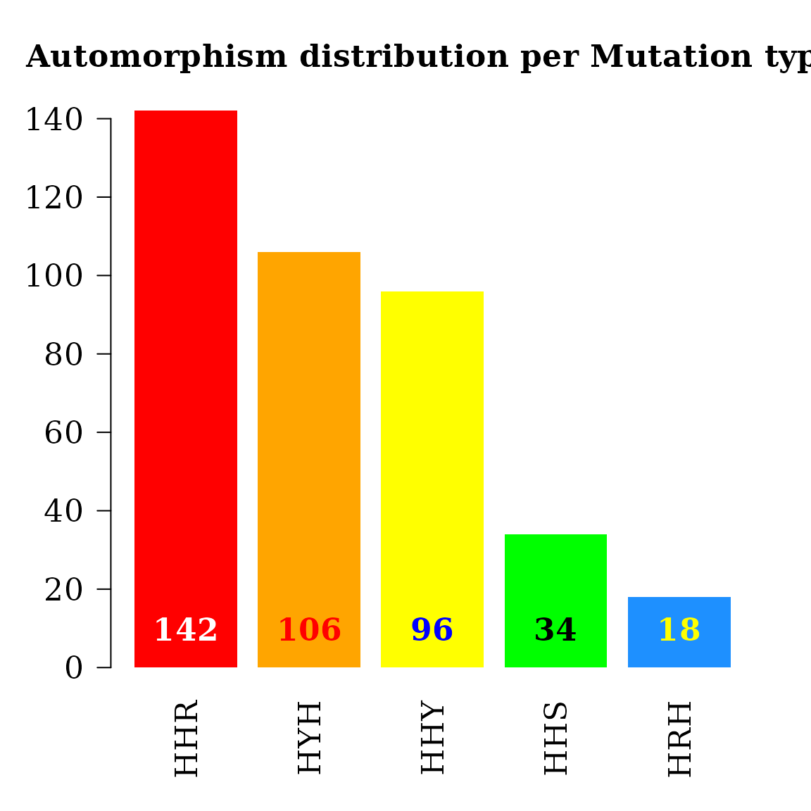
Bar plot automorphism distribution by cubes
The automorphism distribution by cubes can be summarized in the bar-plot graphic.
Object autby_coef carried all the pairwise comparisons, while it will be enough to use data from a single species as reference, e.g., humans.
First the data must be reordered into a object:
hautby_coef <- autby_coef[ grep("human", names(autby_coef)) ]
h_autby_coef <- unlist(hautby_coef)
h_autby_coef <- h_autby_coef[ which(h_autby_coef$autm != 1) ]

nams <- names(h_autby_coef)
nams <- sub("human[_][1-6][.]", "", nams)
nams <- sub("[_][1-6]", "", nams)

dt <- data.frame(h_autby_coef, species = nams)
dt <- dt[, c("start", "autm", "species", "cube")]
Nominal variables are transformed into
dt$start <- as.numeric(dt$start)
dt$autm <- as.numeric(dt$autm)
dt$cube <- as.factor(dt$cube)
dt$species <- as.factor(dt$species)
DataFrame(dt)
#> DataFrame with 282 rows and 4 columns
#>         start      autm   species     cube
#>     <numeric> <numeric>  <factor> <factor>
#> 1          37         3   gorilla     ACGT
#> 2          51        19   human       ACGT
#> 3          61        51   human       TGCA
#> 4          41         3   human       ACGT
#> 5          18        33   human       ACGT
#> ...       ...       ...       ...      ...
#> 278        54        43 orangutan     TGCA
#> 279        16        54 orangutan     ACGT
#> 280        18        33 orangutan     ACGT
#> 281        37         3 orangutan     ACGT
#> 282        54        43 orangutan     TGCA
counts <- table(dt$cube)

par(family = "serif", cex = 0.6, font = 2, mar=c(4,6,4,4))
barplot(counts, #main="Automorphism distribution",
        xlab="Genetic-code cube representation",
        ylab="Fixed mutational events",
        col=c("darkblue","red", "darkgreen", "magenta", "orange"),
        border = NA, axes = F, #ylim = c(0, 6000),
        cex.lab = 2, cex.main = 1.5, cex.names = 2)
axis(2, at = c(0, 50, 100, 150, 200), cex.axis = 1.5)
mtext(side = 1,line = -2.5, at = c(0.7, 1.9, 3.1, 4.3, 5.5),
      text = paste0( counts ), cex = 1.4,
      col = c("white", "yellow"))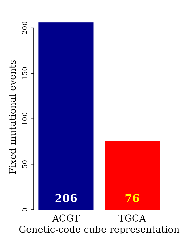
Conserved and non-conserved regions
A specific function is provided to get the coordinates of conserved and non-conserved regions, which can be used in further downstream analyses.
The conserved regions from each pairwise comparison are retrieved typing:
conserved_regions(x = autby_coef)
#> AutomorphismByCoef object with 11023 ranges and 7 metadata columns:
#>                           seqnames    ranges strand |        seq1        seq2         aa1         aa2      autm
#>                              <Rle> <IRanges>  <Rle> | <character> <character> <character> <character> <numeric>
#>       human_1.orangutan_1        1      1-15      + |         ATG         ATG           M           M         1
#>       human_1.orangutan_1        1      1-15      + |         GGT         GGT           G           G         1
#>       human_1.orangutan_1        1      1-15      + |         GAT         GAT           D           D         1
#>       human_1.orangutan_1        1      1-15      + |         GTT         GTT           V           V         1
#>       human_1.orangutan_1        1      1-15      + |         GAG         GAG           E           E         1
#>                       ...      ...       ...    ... .         ...         ...         ...         ...       ...
#>   orangutan_1.orangutan_2        1     1-106      + |         GAC         GAC           D           D         1
#>   orangutan_1.orangutan_2        1     1-106      + |         TTA         TTA           L           L         1
#>   orangutan_1.orangutan_2        1     1-106      + |         ATA         ATA           I           I         1
#>   orangutan_1.orangutan_2        1     1-106      + |         GCT         GCT           A           A         1
#>   orangutan_1.orangutan_2        1     1-106      + |         TAA         TAA           *           *         1
#>                              mut_type        cube
#>                           <character> <character>
#>       human_1.orangutan_1         HHH        ACGT
#>       human_1.orangutan_1         HHH        ACGT
#>       human_1.orangutan_1         HHH        ACGT
#>       human_1.orangutan_1         HHH        ACGT
#>       human_1.orangutan_1         HHH        ACGT
#>                       ...         ...         ...
#>   orangutan_1.orangutan_2         HHH        ACGT
#>   orangutan_1.orangutan_2         HHH        ACGT
#>   orangutan_1.orangutan_2         HHH        ACGT
#>   orangutan_1.orangutan_2         HHH        ACGT
#>   orangutan_1.orangutan_2         HHH        ACGT
#>   -------
#>   seqinfo: 1 sequence from an unspecified genome; no seqlengths
The non-conserved regions from each pairwise comparison are obtained with the same function but different settings:
ncs <- conserved_regions(x = autby_coef, conserved = FALSE)
ncs
#> AutomorphismByCoef object with 396 ranges and 7 metadata columns:
#>                                seqnames    ranges strand |        seq1        seq2         aa1         aa2      autm
#>                                   <Rle> <IRanges>  <Rle> | <character> <character> <character> <character> <numeric>
#>            human_1.orangutan_1        1        16      + |         TCC         TCG           S           S        54
#>            human_1.orangutan_2        1        16      + |         TCC         TCG           S           S        54
#>            human_2.orangutan_1        1        16      + |         TCC         TCG           S           S        54
#>            human_2.orangutan_2        1        16      + |         TCC         TCG           S           S        54
#>            gorilla.orangutan_1        1        16      + |         TCC         TCG           S           S        54
#>                            ...      ...       ...    ... .         ...         ...         ...         ...       ...
#>   rhesus_monkeys_2.orangutan_2        1        95      + |         TTG         TTA           L           L        34
#>    gelada_baboon_1.orangutan_1        1        95      + |         TTG         TTA           L           L        34
#>    gelada_baboon_1.orangutan_2        1        95      + |         TTG         TTA           L           L        34
#>    gelada_baboon_2.orangutan_1        1        95      + |         TTG         TTA           L           L        34
#>    gelada_baboon_2.orangutan_2        1        95      + |         TTG         TTA           L           L        34
#>                                   mut_type        cube
#>                                <character> <character>
#>            human_1.orangutan_1         HHS        ACGT
#>            human_1.orangutan_2         HHS        ACGT
#>            human_2.orangutan_1         HHS        ACGT
#>            human_2.orangutan_2         HHS        ACGT
#>            gorilla.orangutan_1         HHS        ACGT
#>                            ...         ...         ...
#>   rhesus_monkeys_2.orangutan_2         HHR        ACGT
#>    gelada_baboon_1.orangutan_1         HHR        ACGT
#>    gelada_baboon_1.orangutan_2         HHR        ACGT
#>    gelada_baboon_2.orangutan_1         HHR        ACGT
#>    gelada_baboon_2.orangutan_2         HHR        ACGT
#>   -------
#>   seqinfo: 1 sequence from an unspecified genome; no seqlengths
Subsetting regions of interest
The application of some of the available bioinformatic tools is straightforward. For example, knowing the positions for the conserved and non-conserved regions, we can subset into the alignment region of potential interest.
The coordinates carrying mutational events are:
We will use function DNAStringSet from the Bioconductor R package Biostrings to subset the MSA of primate cytochrome c.
cyc_aln_region <- DNAStringSet(cyc_aln, start = 37*3 - 2, end = 42*3)
cyc_aln_region
#> DNAStringSet object of length 19:
#>      width seq                                                                                      names
#>  [1]    18 TTTGGGCGGAAGACAGGT                                                                       NM_018947.6 Homo ...
#>  [2]    18 TTTGGGCGGAAGACAGGT                                                                       gb|BC021994.1|  [...
#>  [3]    18 TTCGGGCGGAAGACAGGT                                                                       ref|XM_019031021....
#>  [4]    18 TTTGGGCGGAAGACAGGT                                                                       dbj|AK311836.1|  ...
#>  [5]    18 TTTGGGCGGAAGACAGGT                                                                       gb|BC067222.1|  [...
#>  ...   ... ...
#> [15]    18 TTCGGGCGGAAGACAGGT                                                                       ref|XM_028845948....
#> [16]    18 TTCGGGCGGAAGACAGGT                                                                       ref|XM_025380676....
#> [17]    18 TTCGGGCGGAAGACAGGT                                                                       ref|XM_025380675....
#> [18]    18 TTCGGGCGGAAGACAGGT                                                                       ref|NM_001131167....
#> [19]    18 TTCGGGCGGAAGACAGGT                                                                       emb|CR857183.1|  ...
Next, function ggseqlogo from the R package ggseqlogo will be applied to get the logo sequence from the selected MSA region.
ggseqlogo( as.character(cyc_aln_region) )
#> Warning: The `<scale>` argument of `guides()` cannot be `FALSE`. Use "none" instead as of ggplot2 3.3.4.
#> ℹ The deprecated feature was likely used in the ggseqlogo package.
#>   Please report the issue at <https://github.com/omarwagih/ggseqlogo/issues>.
#> This warning is displayed once every 8 hours.
#> Call `lifecycle::last_lifecycle_warnings()` to see where this warning was generated.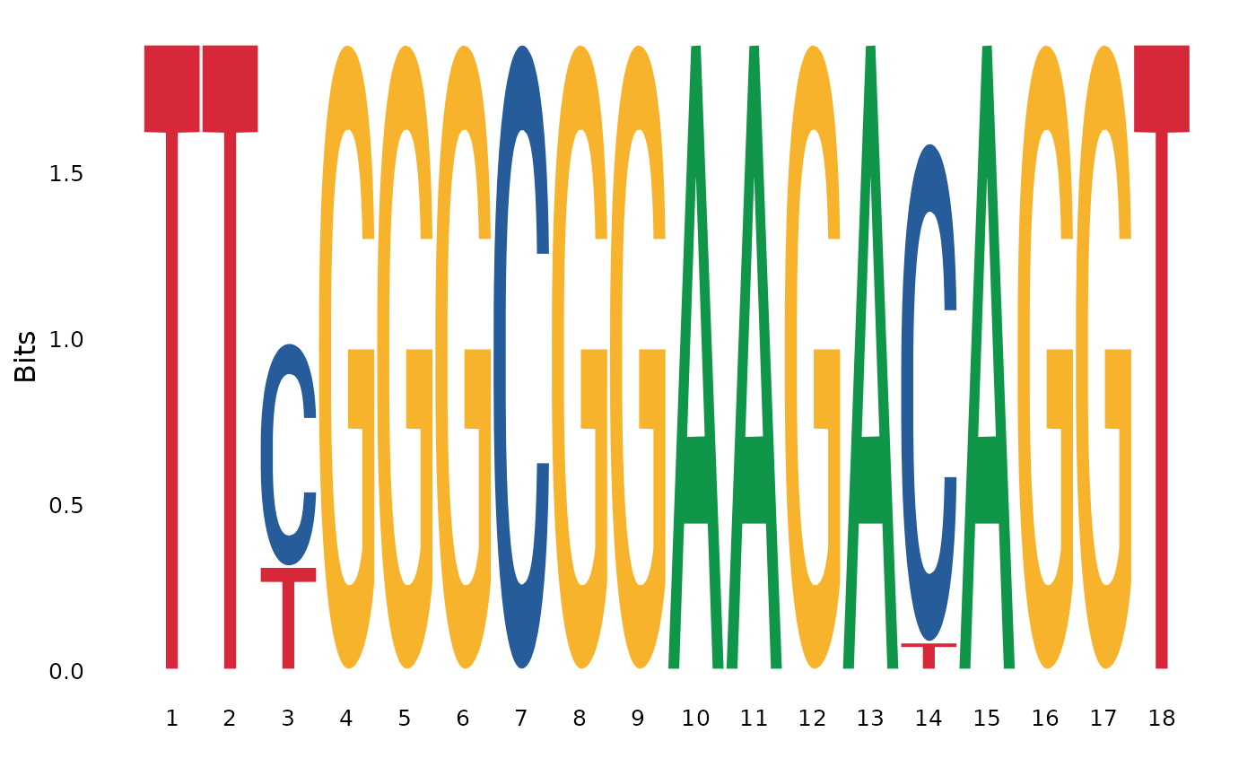
The corresponding aminoacid sequence will be
cyc_aln_region_aa = translate(cyc_aln_region)
cyc_aln_region_aa
#> AAStringSet object of length 19:
#>      width seq                                                                                      names
#>  [1]     6 FGRKTG                                                                                   NM_018947.6 Homo ...
#>  [2]     6 FGRKTG                                                                                   gb|BC021994.1|  [...
#>  [3]     6 FGRKTG                                                                                   ref|XM_019031021....
#>  [4]     6 FGRKTG                                                                                   dbj|AK311836.1|  ...
#>  [5]     6 FGRKTG                                                                                   gb|BC067222.1|  [...
#>  ...   ... ...
#> [15]     6 FGRKTG                                                                                   ref|XM_028845948....
#> [16]     6 FGRKTG                                                                                   ref|XM_025380676....
#> [17]     6 FGRKTG                                                                                   ref|XM_025380675....
#> [18]     6 FGRKTG                                                                                   ref|NM_001131167....
#> [19]     6 FGRKTG                                                                                   emb|CR857183.1|  ...
And the corresponding aminoacid sequence logo will is
ggseqlogo( as.character(cyc_aln_region_aa) )![]()
That is, the first mutational event reported in the codon sequence correspond to a synonymous mutation.
Alternatively, we can start translating the DNA MSA.
cyc_aln_aa <- translate(cyc_aln@unmasked)
cyc_aln_aa
#> AAStringSet object of length 19:
#>      width seq                                                                                      names
#>  [1]   106 MGDVEKGKKIFIMKCSQCHTVEKGGKHKTGPNLHGLFGRKTGQ...LMEYLENPKKYIPGTKMIFVGIKKKEERADLIAYLKKATNE* NM_018947.6 Homo ...
#>  [2]   106 MGDVEKGKKIFIMKCSQCHTVEKGGKHKTGPNLHGLFGRKTGQ...LMEYLENPKKYIPGTKMIFVGIKKKEERADLIAYLKKATNE* gb|BC021994.1|  [...
#>  [3]   106 MGDVEKGKKIFIMKCSQCHTVEKGGKHKTGPNLHGLFGRKTGQ...LMEYLENPKKYIPGTKMIFVGIKKKEERADLIAYLKKATNE* ref|XM_019031021....
#>  [4]   106 MGDVEKGKKIFIMKCSQCHTVEKGGKHKTGPNLHGLFGRKTGQ...LMEYLENPKKYIPGTKMIFVGIKKKEERADLIAYLKKATNE* dbj|AK311836.1|  ...
#>  [5]   106 MGDVEKGKKIFIMKCSQCHTVEKGGKHKTGPNLHGLFGRKTGQ...LMEYLENPKKYIPGTKMIFVGIKKKEERADLIAYLKKATNE* gb|BC067222.1|  [...
#>  ...   ... ...
#> [15]   106 MGDVEKGKKIFIMKCSQCHTVEKGGKHKTGPNLHGLFGRKTGQ...LMEYLENPKKYIPGTKMIFVGIKKKEERADLIAYLKKATNE* ref|XM_028845948....
#> [16]   106 MGDVEKGKKIFIMKCSQCHTVEKGGKHKTGPNLHGLFGRKTGQ...LMEYLENPKKYIPGTKMIFVGIKKKEERADLIAYLKKATNE* ref|XM_025380676....
#> [17]   106 MGDVEKGKKIFIMKCSQCHTVEKGGKHKTGPNLHGLFGRKTGQ...LMEYLENPKKYIPGTKMIFVGIKKKEERADLIAYLKKATNE* ref|XM_025380675....
#> [18]   106 MGDVEKGKKIFIMKCSQCHTVEKGGKHKTGPNLHGLFGRKTGQ...LMEYLENPKKYIPGTKMIFVGIKKKEERADLIAYLKKATNE* ref|NM_001131167....
#> [19]   106 MGDVEKGKKIFIMKCSQCHTVEKGGKHKTGPNLHGLFGRKTGQ...LMEYLENPKKYIPGTKMIFVGIKKKEERADLIAYLKKATNE* emb|CR857183.1|  ...
cyc_aln_aa_region <- AAStringSet(cyc_aln_aa, start = 37, end = 42)
cyc_aln_aa_region
#> AAStringSet object of length 19:
#>      width seq                                                                                      names
#>  [1]     6 FGRKTG                                                                                   NM_018947.6 Homo ...
#>  [2]     6 FGRKTG                                                                                   gb|BC021994.1|  [...
#>  [3]     6 FGRKTG                                                                                   ref|XM_019031021....
#>  [4]     6 FGRKTG                                                                                   dbj|AK311836.1|  ...
#>  [5]     6 FGRKTG                                                                                   gb|BC067222.1|  [...
#>  ...   ... ...
#> [15]     6 FGRKTG                                                                                   ref|XM_028845948....
#> [16]     6 FGRKTG                                                                                   ref|XM_025380676....
#> [17]     6 FGRKTG                                                                                   ref|XM_025380675....
#> [18]     6 FGRKTG                                                                                   ref|NM_001131167....
#> [19]     6 FGRKTG                                                                                   emb|CR857183.1|  ...
ggseqlogo( as.character(cyc_aln_aa_region) )
References
1. Sanchez R, Morgado E, Grau R. Gene algebra from a genetic code algebraic structure. J Math Biol. 2005 Oct;51(4):431-57. doi: 10.1007/s00285-005-0332-8. Epub 2005 Jul 13. PMID: 16012800. ( PDF).
2. Robersy Sanchez, Jesús Barreto (2021) Genomic Abelian Finite Groups. doi: 10.1101/2021.06.01.446543.
3. M. V José, E.R. Morgado, R. Sánchez, T. Govezensky, The 24 possible algebraic representations of the standard genetic code in six or in three dimensions, Adv. Stud. Biol. 4 (2012) 119–152.PDF.
4. R. Sanchez. Symmetric Group of the Genetic–Code Cubes. Effect of the Genetic–Code Architecture on the Evolutionary Process MATCH Commun. Math. Comput. Chem. 79 (2018) 527-560. PDF.