A Short Introduction to Algebraic Taxonomy on Genes Regions. II
Robersy Sanchez
Department of Biology. Pennsylvania State University, University Park, PA 16802rus547@psu.edu
28 December 2024
Source:vignettes/automorphism_and_decision_tree_II.Rmd
automorphism_and_decision_tree_II.RmdAbstract
A fast introduction into the analysis of DNA mutational events by means of automorphisms between two DNA sequences algebraically represented as Abelian finite group. In the current case we propose expressing of the effect of mutational events in terms of distance between codons in the framework set in reference (1). The decision tree is build based on Chi-squared Automated Interaction Detection (CHAID) algorithm.
Overview
This is part II of the tutorial A Short Introduction to Algebraic Taxonomy on Genes Regions
Decision tree
Although the analysis will be accomplish in a dataset with 41 DNA sequences, mostly humans, still the information from other species is poor. So, the conclusion retrieved from the analysis most be taken cautiously, and these are only for illustrative purpose on the application of the theory.
If all the required libraries all installed, then we proceed to load the libraries
library(GenomAutomorphism)
#> Error in get(paste0(generic, ".", class), envir = get_method_env()) :
#>   object 'type_sum.accel' not found
library(Biostrings)
library(party)
library(partykit)
library(data.table)
library(ggplot2)
library(ggparty)
library(dplyr)
library(CHAID)
The dataset carrying 41 aligned DNA sequences of BRCA1 genes from primates is provided with the package.
data(brca1_aln2, package = "GenomAutomorphism")
brca1_aln2
#> DNAMultipleAlignment with 41 rows and 2283 columns
#>       aln                                                                                           names
#>  [1] ATGGATTTATCTGCTCTTCGCGTTGAAGAAGTACAAAATGTCATT...CTGGACACCTACCTGATACCCCAGATCCCCCACAGCCACTACTGA NM_007298.3:20-22...
#>  [2] ATGGATTTATCTGCTCTTCGCGTTGAAGAAGTACAAAATGTCATT...CTGGACACCTACCTGATACCCCAGATCCCCCACAGCCACTACTGA U64805.1:1-2280_H...
#>  [3] ATGGATTTCTCTGCTCTTCGCGTTGAAGAAGTACAAAATGTCATT...CTGGACACCTACCTGATACCCCAGATCCCCCACAGCCACTACTGA NM_007298.3:20-22...
#>  [4] ATGGATTTGTCTGCTCTTCGCGTTGAAGAAGTACAAAATGTCATT...CTGGACACCTACCTGATACCCCAGATCCCCCACAGCCACTACTGA NM_007298.3:20-22...
#>  [5] ATGGATTTTTCTGCTCTTCGCGTTGAAGAAGTACAAAATGTCATT...CTGGACACCTACCTGATACCCCAGATCCCCCACAGCCACTACTGA NM_007298.3:20-22...
#>  [6] ATGGATTTTTCTGCTCTTCGGGTTGAAGAAGTACAAAATGTCATT...CTGGACACCTACCTGATACCCCAGATCCCCCACAGCCACTACTGA NM_007298.3:20-22...
#>  [7] ATGGATTTTTCTGCTCTTCGCTTTGAAGAAGTACAAAATGTCATT...CTGGACACCTACCTGATACCCCAGATCCCCCACAGCCACTACTGA NM_007298.3:20-22...
#>  [8] ATGGATTTTTCTGCTCTTCGCCTTGAAGAAGTACAAAATGTCATT...CTGGACACCTACCTGATACCCCAGATCCCCCACAGCCACTACTGA NM_007298.3:20-22...
#>  [9] ATGGATTTTTCTGCTCTTCGCATTGAAGAAGTACAAAATGTCATT...CTGGACACCTACCTGATACCCCAGATCCCCCACAGCCACTACTGA NM_007298.3:20-22...
#>  ... ...
#> [33] ATGGATTTATCTGCTCTTCGCGTTGAAGAAGTACAAAATGTCATT...CTGGACACCTACCTGATACCTCAGATCCCCCACAGCCACTACTGA XM_034941185.1:24...
#> [34] ATGGATTTATCTGCTCTTCGCGTTGAAGAAGTACAAAATGTCATT...CTGGACACCTACCTGATACCTCAGATCCCCCACAGCCACTACTGA XM_034941182.1:25...
#> [35] ATGGATTTATCTGCTGTTCGCGTTGAAGAAGTACAAAATGTCATT...CTGGATACCTACCTGATACCCCAGATCCCCCACAGCCACTACTGA XM_032163757.1:14...
#> [36] ATGGATTTATCTGCTGTTCGCGTTGAAGAAGTACAAAATGTCATT...CTGGATACCTACCTGATACCCCAGATCCCCCACAGCCACTACTGA XM_032163756.1:14...
#> [37] ATGGATTTATCTGCTGTTCGCGTTGAAGAAGTACAAAATGTCATT...CTGGATACCTACCTGATACCCCAGATCCCCCACAGCCACTACTGA XM_032163758.1:13...
#> [38] ATGGATTTATCTGCTCTTCGCGTTGAAGAAGTACAAAATGTCATT...CTGGACGCCTACCTGATACCCCAGATCCCCCACAGCCACTACTGA XM_030923119.1:18...
#> [39] ATGGATTTATCTGCTCTTCGCGTTGAAGAAGTACAAAATGTCATT...CTGGACGCCTACCTGATACCCCAGATCCCCCACAGCCACTACTGA XM_030923118.1:18...
#> [40] ATGGATTTACCTGCTGTTCGCGTTGAAGAAGTACAAAATGTCATT...CTGGACACCTACCTGATACCCCAGATCCCCCACAGCCACTACTGA XM_025363316.1:14...
#> [41] ATGGATTTATCTGCTGTTCGTGTTGAAGAAGTGCAAAATGTCCTT...CTGGACACCTACCTGATACCCCAGATCCCTCACAGCCACTACTGA XM_039475995.1:49...
The sample names
strtrim(names(brca1_aln2@unmasked), 100)
#>  [1] "NM_007298.3:20-2299_Homo_sapiens_BRCA1_DNA_repair_associated_(BRCA1)_transcript_variant_4_mRNA"
#>  [2] "U64805.1:1-2280_Homo_sapiens_Brca1-delta11b_(Brca1)_mRNA_complete_cds"
#>  [3] "NM_007298.3:20-2299_Homo_sapiens_BRCA1_transcript_variant_4_mRNA_9A-C_L3F_rs780157871"
#>  [4] "NM_007298.3:20-2299_Homo_sapiens_BRCA1_transcript_variant_4_mRNA_9A-G_rs780157871"
#>  [5] "NM_007298.3:20-2299_Homo_sapiens_BRCA1_transcript_variant_4_mRNA_9A-T_L3F_rs780157871"
#>  [6] "NM_007298.3:20-2299_Homo_sapiens_BRCA1_transcript_variant_4_mRNA_21C-G_rs149402012"
#>  [7] "NM_007298.3:20-2299_Homo_sapiens_BRCA1_transcript_variant_4_mRNA_22G-T_V8F_rs528902306"
#>  [8] "NM_007298.3:20-2299_Homo_sapiens_BRCA1_transcript_variant_4_mRNA_22G-C_V8L_rs528902306"
#>  [9] "NM_007298.3:20-2299_Homo_sapiens_BRCA1_transcript_variant_4_mRNA_22G-A_V8I_rs528902306"
#> [10] "NM_007298.3:20-2299_Homo_sapiens_BRCA1_transcript_variant_4_mRNA_75C-T_rs80356839"
#> [11] "NM_007298.3:20-2299_Homo_sapiens_BRCA1_transcript_variant_4_mRNA_999T-A_rs1060915"
#> [12] "NM_007298.3:20-2299_Homo_sapiens_BRCA1_transcript_variant_4_mRNA_985A-C_I329L_rs80357157"
#> [13] "NM_007298.3:20-2299_Homo_sapiens_BRCA1_transcript_variant_4_mRNA_1014C-A_D338E_rs1057523168"
#> [14] "NM_007298.3:20-2299_Homo_sapiens_BRCA1_transcript_variant_4_mRNA_1134A-C_rs1555582589."
#> [15] "NM_007298.3:20-2299_Homo_sapiens_BRCA1_transcript_variant_4_mRNA_1327G-T_D443Y_rs28897691"
#> [16] "NM_007298.3:20-2299_Homo_sapiens_BRCA1_transcript_variant_4_mRNA_1327G-C_D443H_rs28897691"
#> [17] "NM_007298.3:20-2299_Homo_sapiens_BRCA1_transcript_variant_4_mRNA_1327G-A_D443N_rs28897691"
#> [18] "NM_007298.3:20-2299_Homo_sapiens_BRCA1_transcript_variant_4_mRNA_1348T-A_L450M_rs80357431"
#> [19] "NM_007298.3:20-2299_Homo_sapiens_BRCA1_transcript_variant_4_mRNA_2100T-C_rs2050995166"
#> [20] "NM_007298.3:20-2299_Homo_sapiens_BRCA1_transcript_variant_4_mRNA_2102T-G_V701G_rs80356920"
#> [21] "NM_007298.3:20-2299_Homo_sapiens_BRCA1_transcript_variant_4_mRNA_2102T-C_V701A_rs80356920"
#> [22] "NM_007298.3:20-2299_Homo_sapiens_BRCA1_transcript_variant_4_mRNA_2102T-A_V701D_rs80356920"
#> [23] "NM_007298.3:20-2299_Homo_sapiens_BRCA1_transcript_variant_4_mRNA_305C-G_A102G_rs80357190"
#> [24] "XM_031011560.1:233-2515_PREDICTED:_Gorilla_gorilla_gorilla_BRCA1_DNA_repair_associated_(BRCA1)_trans"
#> [25] "XM_031011561.1:233-2512_PREDICTED:_Gorilla_gorilla_gorilla_BRCA1_DNA_repair_associated_(BRCA1)_trans"
#> [26] "XM_031011562.1:163-2442_PREDICTED:_Gorilla_gorilla_gorilla_BRCA1_DNA_repair_associated_(BRCA1)_trans"
#> [27] "XM_009432101.3:276-2555_PREDICTED:_Pan_troglodytes_BRCA1_DNA_repair_associated_(BRCA1)_transcript_va"
#> [28] "XM_009432104.3:371-2650_PREDICTED:_Pan_troglodytes_BRCA1_DNA_repair_associated_(BRCA1)_transcript_va"
#> [29] "XM_016930487.2:371-2650_PREDICTED:_Pan_troglodytes_BRCA1_DNA_repair_associated_(BRCA1)_transcript_va"
#> [30] "XM_009432099.3:371-2653_PREDICTED:_Pan_troglodytes_BRCA1_DNA_repair_associated_(BRCA1)_transcript_va"
#> [31] "XM_034941183.1:254-2533_PREDICTED:_Pan_paniscus_BRCA1_DNA_repair_associated_(BRCA1)_transcript_varia"
#> [32] "XM_034941184.1:254-2533_PREDICTED:_Pan_paniscus_BRCA1_DNA_repair_associated_(BRCA1)_transcript_varia"
#> [33] "XM_034941185.1:248-2527_PREDICTED:_Pan_paniscus_BRCA1_DNA_repair_associated_(BRCA1)_transcript_varia"
#> [34] "XM_034941182.1:254-2536_PREDICTED:_Pan_paniscus_BRCA1_DNA_repair_associated_(BRCA1)_transcript_varia"
#> [35] "XM_032163757.1:145-2418_PREDICTED:_Hylobates_moloch_BRCA1_DNA_repair_associated_(BRCA1)_transcript_v"
#> [36] "XM_032163756.1:145-2421_PREDICTED:_Hylobates_moloch_BRCA1_DNA_repair_associated_(BRCA1)_transcript_v"
#> [37] "XM_032163758.1:139-2412_PREDICTED:_Hylobates_moloch_BRCA1_DNA_repair_associated_(BRCA1)_transcript_v"
#> [38] "XM_030923119.1:184-2463_PREDICTED:_Rhinopithecus_roxellana_BRCA1_DNA_repair_associated_(BRCA1)_trans"
#> [39] "XM_030923118.1:183-2465_PREDICTED:_Rhinopithecus_roxellana_BRCA1_DNA_repair_associated_(BRCA1)_trans"
#> [40] "XM_025363316.1:147-2426_PREDICTED:_Theropithecus_gelada_BRCA1_DNA_repair_associated_(BRCA1)_transcri"
#> [41] "XM_039475995.1:49-2328_PREDICTED:_Saimiri_boliviensis_boliviensis_BRCA1_DNA_repair_associated_(BRCA1"
The automorphisms can be computed as before. For the sake of saving time object brca1_autm2 is included with package
## Do not run it. This is included with package

nams <- c(paste0("human_1.", 0:21),"human_2","gorilla_1","gorilla_2","gorilla_3",
        "chimpanzee_1","chimpanzee_2","chimpanzee_3","chimpanzee_4",
        "bonobos_1","bonobos_2","bonobos_3","bonobos_4","silvery_gibbon_1",
        "silvery_gibbon_1","silvery_gibbon_3","golden_monkey_1",
        "golden_monkey_2","gelada_baboon","bolivian_monkey")

brca1_autm2 <- automorphisms(
                      seqs = brca1_aln2,
                      group = "Z64",
                      cube = c("ACGT", "TGCA"),
                      cube_alt = c("CATG", "GTAC"),
                      nms = nams,
                      verbose = FALSE)
Object brca1_autm2 can be load typing:
data(brca1_autm2, package = "GenomAutomorphism")
brca1_autm2
#> AutomorphismList object of length: 820
#> names(820): human_1.0.human_1.1 human_1.0.human_1.2 human_1.0.human_1.3 ... golden_monkey_2.gelada_baboon golden_monkey_2.bolivian_monkey gelada_baboon.bolivian_monkey
#> -------
#> Automorphism object with 761 ranges and 8 metadata columns:
#>         seqnames    ranges strand |        seq1        seq2         aa1         aa2    coord1    coord2      autm
#>            <Rle> <IRanges>  <Rle> | <character> <character> <character> <character> <numeric> <numeric> <numeric>
#>     [1]        1         1      + |         ATG         ATG           M           M        50        50         1
#>     [2]        1         2      + |         GAT         GAT           D           D        11        11         1
#>     [3]        1         3      + |         TTA         TTA           L           L        60        60         1
#>     [4]        1         4      + |         TCT         TCT           S           S        31        31         1
#>     [5]        1         5      + |         GCT         GCT           A           A        27        27         1
#>     ...      ...       ...    ... .         ...         ...         ...         ...       ...       ...       ...
#>   [757]        1       757      + |         CAC         CAC           H           H         5         5         1
#>   [758]        1       758      + |         AGC         AGC           S           S        33        33         1
#>   [759]        1       759      + |         CAC         CAC           H           H         5         5         1
#>   [760]        1       760      + |         TAC         TAC           Y           Y        13        13         1
#>   [761]        1       761      + |         TGA         TGA           *           *        44        44         1
#>                cube
#>         <character>
#>     [1]        ACGT
#>     [2]        ACGT
#>     [3]        ACGT
#>     [4]        ACGT
#>     [5]        ACGT
#>     ...         ...
#>   [757]        ACGT
#>   [758]        ACGT
#>   [759]        ACGT
#>   [760]        ACGT
#>   [761]        ACGT
#>   -------
#>   seqinfo: 1 sequence from an unspecified genome; no seqlengths
#> ...
#> <819 more DFrame element(s)>
#> Two slots: 'DataList' & 'SeqRanges'
#> -------
As before, we are interested on mutational events in respect to human (as reference).
nams <- names(brca1_autm2)
idx1 <- grep("human_1.", nams)
idx2 <- grep("human_2.", nams)
idx <- union(idx1, idx2)
h_brca1_autm <- unlist(brca1_autm2[ idx ])
h_brca1_autm = h_brca1_autm[ which(h_brca1_autm$autm != 1) ]
h_brca1_autm
#> Automorphism object with 16542 ranges and 8 metadata columns:
#>                           seqnames    ranges strand |        seq1        seq2         aa1         aa2    coord1
#>                              <Rle> <IRanges>  <Rle> | <character> <character> <character> <character> <numeric>
#>       human_1.0.human_1.1        1       239      + |         CAT         CGT           H           R         7
#>       human_1.0.human_1.1        1       253      + |         GCA         GTA           A           V        24
#>       human_1.0.human_1.1        1       323      + |         TCT         CCT           S           P        31
#>       human_1.0.human_1.1        1       333      + |         TCT         TCC           S           S        31
#>       human_1.0.human_1.1        1       350      + |         ---         ---           -           -        NA
#>                       ...      ...       ...    ... .         ...         ...         ...         ...       ...
#>   human_2.bolivian_monkey        1       716      + |         AAT         AGT           N           S         3
#>   human_2.bolivian_monkey        1       726      + |         GAG         GAA           E           E        10
#>   human_2.bolivian_monkey        1       730      + |         GTG         GTA           V           V        58
#>   human_2.bolivian_monkey        1       731      + |         ACC         ACT           T           T        17
#>   human_2.bolivian_monkey        1       756      + |         CCC         CCT           P           P        21
#>                              coord2      autm        cube
#>                           <numeric> <numeric> <character>
#>       human_1.0.human_1.1        39        33        ACGT
#>       human_1.0.human_1.1        56        21        ACGT
#>       human_1.0.human_1.1        23         9        ACGT
#>       human_1.0.human_1.1        29         3        ACGT
#>       human_1.0.human_1.1        NA        -1        Gaps
#>                       ...       ...       ...         ...
#>   human_2.bolivian_monkey        35        33        ACGT
#>   human_2.bolivian_monkey         8        52        ACGT
#>   human_2.bolivian_monkey        56        12        ACGT
#>   human_2.bolivian_monkey        19        35        ACGT
#>   human_2.bolivian_monkey        23        59        ACGT
#>   -------
#>   seqinfo: 1 sequence from an unspecified genome; no seqlengths
Autmorphism Grouping by Coefficient
The automorphism distribution by cubes can be summarized in the bar-plot graphic.
Object autby_coef carried all the pairwise comparisons, while it will be enough to use data from a single species as reference, e.g., humans.
First the data must be reordered into a object:
h_autby_coef <- automorphism_bycoef(x = h_brca1_autm)
h_autby_coef
#> AutomorphismByCoef object with 16515 ranges and 7 metadata columns:
#>                              seqnames    ranges strand |        seq1        seq2         aa1         aa2      autm
#>                                 <Rle> <IRanges>  <Rle> | <character> <character> <character> <character> <numeric>
#>          human_1.0.human_1.2        1         3      + |         TTA         TTC           L           F        22
#>          human_1.0.human_1.3        1         3      + |         TTA         TTG           L           L        43
#>          human_1.0.human_1.4        1         3      + |         TTA         TTT           L           F         0
#>          human_1.0.human_1.5        1         3      + |         TTA         TTT           L           F         0
#>          human_1.0.human_1.6        1         3      + |         TTA         TTT           L           F         0
#>                          ...      ...       ...    ... .         ...         ...         ...         ...       ...
#>   human_1.18.bolivian_monkey        1       756      + |         CCC         CCT           P           P        59
#>   human_1.19.bolivian_monkey        1       756      + |         CCC         CCT           P           P        59
#>   human_1.20.bolivian_monkey        1       756      + |         CCC         CCT           P           P        59
#>   human_1.21.bolivian_monkey        1       756      + |         CCC         CCT           P           P        59
#>      human_2.bolivian_monkey        1       756      + |         CCC         CCT           P           P        59
#>                                 mut_type        cube
#>                              <character> <character>
#>          human_1.0.human_1.2         HHM        TGCA
#>          human_1.0.human_1.3         HHR        TGCA
#>          human_1.0.human_1.4         HHW        Trnl
#>          human_1.0.human_1.5         HHW        Trnl
#>          human_1.0.human_1.6         HHW        Trnl
#>                          ...         ...         ...
#>   human_1.18.bolivian_monkey         HHY        ACGT
#>   human_1.19.bolivian_monkey         HHY        ACGT
#>   human_1.20.bolivian_monkey         HHY        ACGT
#>   human_1.21.bolivian_monkey         HHY        ACGT
#>      human_2.bolivian_monkey         HHY        ACGT
#>   -------
#>   seqinfo: 1 sequence from an unspecified genome; no seqlengths
The counts by type of mutations
table(h_autby_coef$mut_type)
#>
#>  ---  HHH  HHK  HHM  HHR  HHS  HHW  HHY  HKH  HMH  HMR  HRH  HRR  HRW  HRY  HSH  HWH  HYH  HYS  KHH  KKH  KWH  KYH  MHH
#>  575  391  290  447 2050  270  769 2358  126  829  253 1648   69    3   46  271  195  626   46  179    3    3    3  573
#>  RHH  RKH  RMH  RWH  RYH  SHH  SHM  WHH  WHK  YHH  YRH  YRY
#> 2469    1   46    1    1  874    1  229   23  755   69   23
Simplifying species names
nams <- names(h_autby_coef)
nams <- sub("human[_][1-2][.]", "", nams)
nams <- sub("[_][1-6]", "", nams)
nams <- sub("[0123456789]*[.]", "", nams)
nams <- sub("[.][0123456789]*", "", nams)

dt <- data.frame(h_autby_coef, species = nams)
dt <- data.frame(dt, species = nams)
dt <- dt[, c("start", "autm", "species", "mut_type", "aa1", "aa2", "cube")]
DataFrame(dt)
#> DataFrame with 16515 rows and 7 columns
#>           start      autm         species    mut_type         aa1         aa2        cube
#>       <integer> <numeric>     <character> <character> <character> <character> <character>
#> 1             3        22           human         HHM           L           F        TGCA
#> 2             3        43           human         HHR           L           L        TGCA
#> 3             3         0           human         HHW           L           F        Trnl
#> 4             3         0           human         HHW           L           F        Trnl
#> 5             3         0           human         HHW           L           F        Trnl
#> ...         ...       ...             ...         ...         ...         ...         ...
#> 16511       756        59 bolivian_monkey         HHY           P           P        ACGT
#> 16512       756        59 bolivian_monkey         HHY           P           P        ACGT
#> 16513       756        59 bolivian_monkey         HHY           P           P        ACGT
#> 16514       756        59 bolivian_monkey         HHY           P           P        ACGT
#> 16515       756        59 bolivian_monkey         HHY           P           P        ACGT
Nominal variables are transformed into
dt$start <- as.numeric(dt$start)
dt$autm <- as.numeric(dt$autm)
dt$cube <- as.factor(dt$cube)
dt$species <- as.factor(dt$species)
dt$mut_type <- as.factor(dt$mut_type)
CHAID using aminoacid/codon distance
In this analysis a new variable has been include, which derives from the estimation of the distance between aminoacids, estimated as suggested in reference (1). The mutational effect is measured in terms of the average of two aminoacid distance functions, which are based on the codon distance.
interval <- function(x, a, b) {
    x >= a & x <= b
}

datos = dt

datos$mut_cost <- round((aminoacid_dist(aa1 = h_autby_coef, group = "Z5",
                               cube = "TCGA" , num.cores = 20) +
                      aminoacid_dist(aa1 = h_autby_coef,
                            weight = c(0.3, 0.9, 0.08), group = "Z5",
                              cube = "TCGA" , num.cores = 20))/2, 2)

hist(datos$mut_cost,10)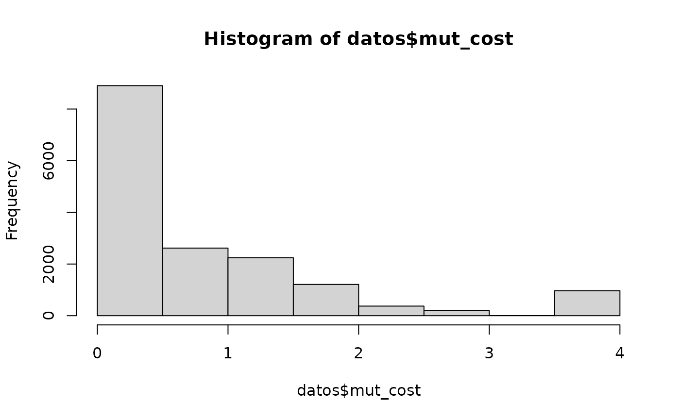
datos$mut_cost[ is.na(datos$mut_cost) ] <- -10


datos$autms <- case_when(datos$autm < 16 ~ 'A1',
                    interval(datos$autm, 16, 31) ~ 'A2',
                    interval(datos$autm, 32, 47) ~ 'A3',
                    datos$autm > 47 ~ 'A4')
datos$autms <- as.factor(datos$autms)

datos$mut_type <- as.character(datos$mut_type)
datos$mut_type <- as.factor(datos$mut_type)

datos$regions <- case_when(datos$start < 102 ~ 'R0',
                    interval(datos$start, 103, 229) ~ 'R0.',
                    interval(datos$start, 230, 270) ~ 'R1',
                    interval(datos$start, 271, 305) ~ 'R2',
                    interval(datos$start, 306, 338) ~ 'R3',
                    interval(datos$start, 339, 533) ~ 'R4',
                    interval(datos$start, 534, 570) ~ 'R5',
                    interval(datos$start, 571, 653) ~ 'R6',
                    interval(datos$start, 654, 709) ~ 'R7',
                    datos$start > 709 ~ 'R8')

datos$regions <- as.factor(datos$regions)

datos$autm <- as.factor(datos$autm)
datos$species <- as.factor(datos$species)
datos$start <- as.factor(datos$start)
datos$cube <- as.factor(datos$cube)
datos$mut_cost <- as.factor(datos$mut_cost)

datos <- datos[, c( "autms", "regions", "mut_type", "cube", "mut_cost", "species")]
DataFrame(datos)
#> DataFrame with 16515 rows and 6 columns
#>          autms  regions mut_type     cube mut_cost         species
#>       <factor> <factor> <factor> <factor> <factor>        <factor>
#> 1           A2       R0      HHM     TGCA     0.26           human
#> 2           A3       R0      HHR     TGCA     0.22           human
#> 3           A1       R0      HHW     Trnl     0.26           human
#> 4           A1       R0      HHW     Trnl     0.26           human
#> 5           A1       R0      HHW     Trnl     0.26           human
#> ...        ...      ...      ...      ...      ...             ...
#> 16511       A4       R8      HHY     ACGT      0.1 bolivian_monkey
#> 16512       A4       R8      HHY     ACGT      0.1 bolivian_monkey
#> 16513       A4       R8      HHY     ACGT      0.1 bolivian_monkey
#> 16514       A4       R8      HHY     ACGT      0.1 bolivian_monkey
#> 16515       A4       R8      HHY     ACGT      0.1 bolivian_monkey
The histogram shows an expected result for a variable measuring the mutational effect: the frequency of mutational events must (exponentially) decrease with the magnitude of the mutational effect.
A classification tree is estimated with CHAID algorithm:
ctrl <- chaid_control(minsplit = 500, minprob = 0.9, alpha2 = 0.01, alpha4 = 0.01)
chaid_res <- chaid(species ~ autms + regions + mut_type + cube + mut_cost,
                   data = datos,  control = ctrl)
chaid_res
#>
#> Model formula:
#> species ~ autms + regions + mut_type + cube + mut_cost
#>
#> Fitted party:
#> [1] root
#> |   [2] mut_cost in 0.06
#> |   |   [3] regions in R0, R5: bolivian_monkey (n = 220, err = 68.6%)
#> |   |   [4] regions in R0.: bolivian_monkey (n = 253, err = 45.5%)
#> |   |   [5] regions in R1: golden_monkey (n = 230, err = 60.0%)
#> |   |   [6] regions in R2: bolivian_monkey (n = 115, err = 40.0%)
#> |   |   [7] regions in R3: gelada_baboon (n = 23, err = 0.0%)
#> |   |   [8] regions in R4
#> |   |   |   [9] autms in A1, A3: golden_monkey (n = 322, err = 57.1%)
#> |   |   |   [10] autms in A2: golden_monkey (n = 276, err = 66.7%)
#> |   |   |   [11] autms in A4: gorilla (n = 92, err = 25.0%)
#> |   |   [12] regions in R6: silvery_gibbon (n = 69, err = 0.0%)
#> |   |   [13] regions in R7: silvery_gibbon (n = 187, err = 61.5%)
#> |   |   [14] regions in R8: silvery_gibbon (n = 89, err = 25.8%)
#> |   [15] mut_cost in 0.1
#> |   |   [16] regions in R0, R2: golden_monkey (n = 243, err = 62.1%)
#> |   |   [17] regions in R0.: bonobos (n = 322, err = 71.4%)
#> |   |   [18] regions in R1: gorilla (n = 69, err = 0.0%)
#> |   |   [19] regions in R3: golden_monkey (n = 69, err = 33.3%)
#> |   |   [20] regions in R4: silvery_gibbon (n = 407, err = 65.4%)
#> |   |   [21] regions in R5, R7: bolivian_monkey (n = 135, err = 31.1%)
#> |   |   [22] regions in R6: bolivian_monkey (n = 138, err = 66.7%)
#> |   |   [23] regions in R8: bonobos (n = 319, err = 71.2%)
#> |   [24] mut_cost in 0.12, 0.35
#> |   |   [25] regions in R0, R6, R7, R8: silvery_gibbon (n = 223, err = 67.7%)
#> |   |   [26] regions in R0.: bolivian_monkey (n = 46, err = 0.0%)
#> |   |   [27] regions in R1, R5: silvery_gibbon (n = 135, err = 0.0%)
#> |   |   [28] regions in R2: golden_monkey (n = 69, err = 33.3%)
#> |   |   [29] regions in R3: human (n = 40, err = 45.0%)
#> |   |   [30] regions in R4: bolivian_monkey (n = 115, err = 60.0%)
#> |   [31] mut_cost in 0.22
#> |   |   [32] regions in R0, R1, R3, R8: golden_monkey (n = 164, err = 70.7%)
#> |   |   [33] regions in R0.: silvery_gibbon (n = 138, err = 50.0%)
#> |   |   [34] regions in R2: golden_monkey (n = 138, err = 33.3%)
#> |   |   [35] regions in R4: bolivian_monkey (n = 161, err = 42.9%)
#> |   |   [36] regions in R5: bolivian_monkey (n = 46, err = 0.0%)
#> |   |   [37] regions in R6: golden_monkey (n = 92, err = 50.0%)
#> |   |   [38] regions in R7: gelada_baboon (n = 23, err = 0.0%)
#> |   [39] mut_cost in 0.26
#> |   |   [40] autms in A1, A2: human (n = 424, err = 71.5%)
#> |   |   [41] autms in A3: silvery_gibbon (n = 93, err = 22.6%)
#> |   |   [42] autms in A4: golden_monkey (n = 92, err = 0.0%)
#> |   [43] mut_cost in 0.28, 1.23
#> |   |   [44] regions in R0, R3, R6, R7, R8: golden_monkey (n = 276, err = 66.7%)
#> |   |   [45] regions in R0.: bonobos (n = 115, err = 20.0%)
#> |   |   [46] regions in R1: bolivian_monkey (n = 23, err = 0.0%)
#> |   |   [47] regions in R2: bonobos (n = 414, err = 77.8%)
#> |   |   [48] regions in R4
#> |   |   |   [49] autms in A1: golden_monkey (n = 162, err = 43.2%)
#> |   |   |   [50] autms in A2: human (n = 42, err = 71.4%)
#> |   |   |   [51] autms in A3: bonobos (n = 488, err = 81.1%)
#> |   |   |   [52] autms in A4: human (n = 14, err = 0.0%)
#> |   |   [53] regions in R5: golden_monkey (n = 161, err = 42.9%)
#> |   [54] mut_cost in 0.31: golden_monkey (n = 184, err = 50.0%)
#> |   [55] mut_cost in 0.32
#> |   |   [56] regions in R0, R0., R3: bonobos (n = 111, err = 20.7%)
#> |   |   [57] regions in R1: chimpanzee (n = 326, err = 71.8%)
#> |   |   [58] regions in R2: golden_monkey (n = 69, err = 33.3%)
#> |   |   [59] regions in R4: silvery_gibbon (n = 184, err = 62.5%)
#> |   |   [60] regions in R5, R7: bolivian_monkey (n = 46, err = 0.0%)
#> |   |   [61] regions in R6: gorilla (n = 138, err = 50.0%)
#> |   |   [62] regions in R8: golden_monkey (n = 46, err = 0.0%)
#> |   [63] mut_cost in 0.33: golden_monkey (n = 448, err = 58.5%)
#> |   [64] mut_cost in 0.41: silvery_gibbon (n = 150, err = 54.0%)
#> |   [65] mut_cost in 0.47, 0.81: bolivian_monkey (n = 46, err = 0.0%)
#> |   [66] mut_cost in 0.53: gorilla (n = 338, err = 78.7%)
#> |   [67] mut_cost in 0.58, 0.78, 1.02: golden_monkey (n = 454, err = 69.6%)
#> |   [68] mut_cost in 0.63: golden_monkey (n = 109, err = 56.0%)
#> |   [69] mut_cost in 0.67: golden_monkey (n = 109, err = 56.0%)
#> |   [70] mut_cost in 0.73, 0.82, 1.52, 2.48: silvery_gibbon (n = 300, err = 53.0%)
#> |   [71] mut_cost in 0.89: bolivian_monkey (n = 184, err = 50.0%)
#> |   [72] mut_cost in 0.94, 1.03: golden_monkey (n = 276, err = 50.0%)
#> |   [73] mut_cost in 0.98: bolivian_monkey (n = 207, err = 66.7%)
#> |   [74] mut_cost in 0.99
#> |   |   [75] regions in R0, R0., R6, R8: bonobos (n = 414, err = 77.8%)
#> |   |   [76] regions in R1: golden_monkey (n = 69, err = 33.3%)
#> |   |   [77] regions in R2: golden_monkey (n = 92, err = 50.0%)
#> |   |   [78] regions in R3: human (n = 79, err = 45.6%)
#> |   |   [79] regions in R4, R7: golden_monkey (n = 299, err = 53.8%)
#> |   |   [80] regions in R5: bolivian_monkey (n = 23, err = 0.0%)
#> |   [81] mut_cost in 1.01: golden_monkey (n = 207, err = 55.6%)
#> |   [82] mut_cost in 1.11, 1.28: bolivian_monkey (n = 93, err = 49.5%)
#> |   [83] mut_cost in 1.12, 1.89, 2.88: gorilla (n = 224, err = 67.9%)
#> |   [84] mut_cost in 1.18: bonobos (n = 256, err = 64.1%)
#> |   [85] mut_cost in 1.19: bolivian_monkey (n = 23, err = 0.0%)
#> |   [86] mut_cost in 1.21
#> |   |   [87] regions in R0, R0., R1, R2, R3, R5, R6, R8: golden_monkey (n = 129, err = 62.8%)
#> |   |   [88] regions in R4: bonobos (n = 414, err = 77.8%)
#> |   |   [89] regions in R7: bolivian_monkey (n = 23, err = 0.0%)
#> |   [90] mut_cost in 1.34: bonobos (n = 437, err = 78.9%)
#> |   [91] mut_cost in 1.36: gorilla (n = 69, err = 0.0%)
#> |   [92] mut_cost in 1.58, 3.38: silvery_gibbon (n = 95, err = 27.4%)
#> |   [93] mut_cost in 1.98
#> |   |   [94] regions in R0, R0., R2, R3, R5, R8: bonobos (n = 460, err = 80.0%)
#> |   |   [95] regions in R1: silvery_gibbon (n = 161, err = 57.1%)
#> |   |   [96] regions in R4: silvery_gibbon (n = 368, err = 43.8%)
#> |   |   [97] regions in R6: golden_monkey (n = 69, err = 33.3%)
#> |   |   [98] regions in R7: human (n = 35, err = 40.0%)
#> |   [99] mut_cost in 2.12, 3.17: golden_monkey (n = 70, err = 34.3%)
#> |   [100] mut_cost in 2.14: bolivian_monkey (n = 230, err = 70.0%)
#> |   [101] mut_cost in 2.22, 2.23: bolivian_monkey (n = 70, err = 32.9%)
#> |   [102] mut_cost in 2.92: golden_monkey (n = 80, err = 42.5%)
#> |   [103] mut_cost in 2.99: bolivian_monkey (n = 23, err = 0.0%)
#> |   [104] mut_cost in 4
#> |   |   [105] mut_type in ---, HHK, HHM, HHR, HHS, HHW, HHY, HKH, HMH, HMR, HRH, HRR, HRW, HRY, HSH, HWH, HYH, HYS, KHH, KKH, KWH, KYH, MHH, RHH, RKH, RMH, RWH, RYH, SHH, SHM, WHH, WHK, YHH, YRH, YRY
#> |   |   |   [106] regions in R0, R0., R1, R3, R5, R6, R7, R8: silvery_gibbon (n = 253, err = 36.4%)
#> |   |   |   [107] regions in R2: bonobos (n = 23, err = 0.0%)
#> |   |   |   [108] regions in R4: bonobos (n = 299, err = 76.9%)
#> |   |   [109] mut_type in HHH: human (n = 391, err = 35.3%)
#>
#> Number of inner nodes:    15
#> Number of terminal nodes: 94
Plotting the CHAID tree (II)
Next, the data must be prepared for plotting the tree with ggparty:
##  Updating CHAID decision tree
dp <- data_party(chaid_res)
dat <- dp[, c("autms", "regions", "mut_type", "mut_cost")]
dat$species <- dp[, "(response)"]


chaid_tree <- party(node = node_party(chaid_res),
                    data = dat,
                    fitted =  dp[, c("(fitted)", "(response)")],
                    names = names(chaid_res))

## Extract p-values
pvals <- unlist(nodeapply(chaid_tree, ids = nodeids(chaid_tree), function(n) {
    pvals <- info_node(n)$adjpvals
    pvals < pvals[ which.min(pvals) ]
    return(pvals)
}))
pvals <- pvals[ pvals < 0.05 ]

## Counts of event per spciees on each node
node.freq <- sapply(seq_along(chaid_tree), function(id) {
    y <- data_party(chaid_tree, id = id)
    y <- y[[ "(response)" ]]
    table(y)
})
## total counts on each
node.size =  colSums(node.freq)
Plotting the tree with ggparty (font size adjusted for html output)
ggparty(chaid_tree, horizontal = TRUE) +
    geom_edge(aes(color = id, size = node.size[id]/300), show.legend = FALSE) +
    geom_edge_label(size = 12, colour = "red",
                    fontface = "bold",
                    shift = 0.64,
                    nudge_x = -0.01,
                    max_length = 10,
                    splitlevels = 1:4) +
    geom_node_label(line_list = list(aes(label = paste0("Node ", id, ": ", splitvar)),
                aes(label = paste0("N=", node.size[id], ", p",
                                 ifelse(pvals < .001, "<.001",
                                        paste0("=", round(pvals, 3)))),
                    size = 30)),
                    line_gpar = list(list(size = 30),
                                     list(size = 30)),
                ids = "inner", fontface = "bold", size = 30) +
    geom_node_info() +
    geom_node_label(aes(label = paste0("N = ", node.size),
                        fontface = "bold"),
                    ids = "terminal", nudge_y = -0.0, nudge_x = 0.01, size = 12) +
    geom_node_plot(gglist = list(
        geom_bar(aes(x = "", fill = species), size = 0.7, width = 0.9,
                 position = position_fill(), color = "black"),
        theme_minimal(base_family = "arial", base_size = 20),
        theme(legend.key.size = unit(2, "cm"),
              legend.key.width = unit(3.5, 'cm'),
              legend.text = element_text(size = 50),
              legend.title = element_text(size = 52),
              text = element_text(size = 44)),
        coord_flip(),
        scale_fill_manual(values = c("gray50","gray55","gray60",
                                     "gray70","gray80","gray85",
                                     "dodgerblue","gray95")),
        xlab(""),
        ylab("Probability"),
        geom_text(aes(x = "", group = species,
                      label = stat(count)),
                  stat = "count", position = position_fill(),
                  vjust = 0.6, hjust = 1.5, size = 14)),
        shared_axis_labels = TRUE, size = 1.4)
It is important to observe that, as shown in reference (1), that the optimal weights applied to compute the aminoacid distances can be estimated for each gene or genomic region via genetic algorithm. The optimization takes place by simulating the mutational process in the corresponding gene/region population.
Stochastic-deterministic logical rules
Since only one mutational event human-to-human in region R1 from class A3 is reported in the right side of the tree, with high probability only non-humans hold the following rule:
rule <- (dat$mut_cost == 1.34 )
table(as.character(dat[rule,]$species))
#>
#> bolivian_monkey         bonobos      chimpanzee   gelada_baboon   golden_monkey  silvery_gibbon
#>              46              92              92              46              92              69
Only humans-to-human mutations hold the following rule:
rule <- (dat$mut_cost == 0.28 & dat$regions == "R4" & dat$autm == "A4")
table(as.character(dat[ rule, ]$species))
#>
#> human
#>    14
Only gorilla hold the following rule
rule <- (dat$mut_cost == 1.36 )
table(as.character(dat[rule,]$species))
#>
#> gorilla
#>      69
Only Bolivian monkey holds:
rule <- ((dat$mut_cost == 0.12 | dat$mut_cost == 0.35) & (dat$regions == "R1" | dat$regions == "R5"))
table(as.character(dat[rule,]$species))
#>
#> silvery_gibbon
#>            135
CHAID with different model
ctrl <- chaid_control(minsplit = 200, minprob = 0.9, alpha2 = 0.01, alpha4 = 0.05)
chaid_res <- chaid(species ~ autms + regions + mut_type + mut_cost,
                   data = datos,  control = ctrl)
chaid_res
#>
#> Model formula:
#> species ~ autms + regions + mut_type + mut_cost
#>
#> Fitted party:
#> [1] root
#> |   [2] mut_cost in 0.06
#> |   |   [3] regions in R0, R5
#> |   |   |   [4] autms in A1: silvery_gibbon (n = 69, err = 0.0%)
#> |   |   |   [5] autms in A2: gorilla (n = 92, err = 25.0%)
#> |   |   |   [6] autms in A3: human (n = 13, err = 0.0%)
#> |   |   |   [7] autms in A4: bolivian_monkey (n = 46, err = 0.0%)
#> |   |   [8] regions in R0.
#> |   |   |   [9] autms in A1, A4: bolivian_monkey (n = 46, err = 0.0%)
#> |   |   |   [10] autms in A2: bolivian_monkey (n = 138, err = 50.0%)
#> |   |   |   [11] autms in A3: golden_monkey (n = 69, err = 33.3%)
#> |   |   [12] regions in R1
#> |   |   |   [13] autms in A1, A4: golden_monkey (n = 46, err = 0.0%)
#> |   |   |   [14] autms in A2: golden_monkey (n = 69, err = 33.3%)
#> |   |   |   [15] autms in A3: silvery_gibbon (n = 115, err = 40.0%)
#> |   |   [16] regions in R2: bolivian_monkey (n = 115, err = 40.0%)
#> |   |   [17] regions in R3: gelada_baboon (n = 23, err = 0.0%)
#> |   |   [18] regions in R4
#> |   |   |   [19] autms in A1, A3: golden_monkey (n = 322, err = 57.1%)
#> |   |   |   [20] autms in A2
#> |   |   |   |   [21] mut_type in ---, HHH, HHK, HHM, HHR, HHS, HHW, HKH, HMH, HMR, HRH, HRR, HRW, HRY, HSH, HWH, HYH, HYS, KHH, KKH, KWH, KYH, MHH, RHH, RKH, RMH, RWH, RYH, SHH, SHM, WHH, WHK, YHH, YRH, YRY: golden_monkey (n = 253, err = 63.6%)
#> |   |   |   |   [22] mut_type in HHY: bolivian_monkey (n = 23, err = 0.0%)
#> |   |   |   [23] autms in A4: gorilla (n = 92, err = 25.0%)
#> |   |   [24] regions in R6: silvery_gibbon (n = 69, err = 0.0%)
#> |   |   [25] regions in R7: silvery_gibbon (n = 187, err = 61.5%)
#> |   |   [26] regions in R8: silvery_gibbon (n = 89, err = 25.8%)
#> |   [27] mut_cost in 0.1
#> |   |   [28] regions in R0, R2
#> |   |   |   [29] autms in A1, A3: golden_monkey (n = 184, err = 50.0%)
#> |   |   |   [30] autms in A2: bolivian_monkey (n = 23, err = 0.0%)
#> |   |   |   [31] autms in A4: human (n = 36, err = 38.9%)
#> |   |   [32] regions in R0.
#> |   |   |   [33] mut_type in ---, HHH, HHK, HHM, HHW, HKH, HMH, HMR, HRH, HRR, HRW, HRY, HSH, HWH, HYH, HYS, KHH, KKH, KWH, KYH, MHH, RHH, RKH, RMH, RWH, RYH, SHH, SHM, WHH, WHK, YHH, YRH, YRY: bolivian_monkey (n = 23, err = 0.0%)
#> |   |   |   [34] mut_type in HHR: gelada_baboon (n = 23, err = 0.0%)
#> |   |   |   [35] mut_type in HHS: silvery_gibbon (n = 92, err = 25.0%)
#> |   |   |   [36] mut_type in HHY: bonobos (n = 184, err = 50.0%)
#> |   |   [37] regions in R1: gorilla (n = 69, err = 0.0%)
#> |   |   [38] regions in R3: golden_monkey (n = 69, err = 33.3%)
#> |   |   [39] regions in R4
#> |   |   |   [40] mut_type in ---, HHH, HHK, HHS, HHY, HKH, HMH, HMR, HRH, HRR, HRW, HRY, HSH, HWH, HYH, HYS, KHH, KKH, KWH, KYH, MHH, RHH, RKH, RMH, RWH, RYH, SHH, SHM, WHH, WHK, YHH, YRH, YRY: gelada_baboon (n = 23, err = 0.0%)
#> |   |   |   [41] mut_type in HHM: golden_monkey (n = 85, err = 43.5%)
#> |   |   |   [42] mut_type in HHR: golden_monkey (n = 69, err = 33.3%)
#> |   |   |   [43] mut_type in HHW
#> |   |   |   |   [44] autms in A1, A2, A3: silvery_gibbon (n = 161, err = 57.1%)
#> |   |   |   |   [45] autms in A4: silvery_gibbon (n = 69, err = 0.0%)
#> |   |   [46] regions in R5, R7: bolivian_monkey (n = 135, err = 31.1%)
#> |   |   [47] regions in R6: bolivian_monkey (n = 138, err = 66.7%)
#> |   |   [48] regions in R8
#> |   |   |   [49] autms in A1, A2, A3: bolivian_monkey (n = 46, err = 0.0%)
#> |   |   |   [50] autms in A4: bonobos (n = 273, err = 66.3%)
#> |   [51] mut_cost in 0.12, 0.35
#> |   |   [52] regions in R0, R6, R7, R8
#> |   |   |   [53] mut_type in ---, HHH, HHK, HHM, HHR, HHW, HKH, HMH, HMR, HRH, HRR, HRW, HRY, HSH, HWH, HYH, HYS, KHH, KKH, KWH, KYH, MHH, RHH, RKH, RMH, RWH, RYH, SHH, SHM, WHH, WHK, YHH, YRH, YRY: silvery_gibbon (n = 162, err = 57.4%)
#> |   |   |   [54] mut_type in HHS: human (n = 39, err = 43.6%)
#> |   |   |   [55] mut_type in HHY: bolivian_monkey (n = 22, err = 0.0%)
#> |   |   [56] regions in R0.: bolivian_monkey (n = 46, err = 0.0%)
#> |   |   [57] regions in R1, R5: silvery_gibbon (n = 135, err = 0.0%)
#> |   |   [58] regions in R2: golden_monkey (n = 69, err = 33.3%)
#> |   |   [59] regions in R3: human (n = 40, err = 45.0%)
#> |   |   [60] regions in R4: bolivian_monkey (n = 115, err = 60.0%)
#> |   [61] mut_cost in 0.22
#> |   |   [62] regions in R0, R1, R3, R8: golden_monkey (n = 164, err = 70.7%)
#> |   |   [63] regions in R0.: silvery_gibbon (n = 138, err = 50.0%)
#> |   |   [64] regions in R2: golden_monkey (n = 138, err = 33.3%)
#> |   |   [65] regions in R4: bolivian_monkey (n = 161, err = 42.9%)
#> |   |   [66] regions in R5: bolivian_monkey (n = 46, err = 0.0%)
#> |   |   [67] regions in R6: golden_monkey (n = 92, err = 50.0%)
#> |   |   [68] regions in R7: gelada_baboon (n = 23, err = 0.0%)
#> |   [69] mut_cost in 0.26
#> |   |   [70] autms in A1, A2
#> |   |   |   [71] regions in R0, R1, R2, R3, R4, R5, R6, R7, R8
#> |   |   |   |   [72] regions in R0, R0., R1, R2, R3, R5, R6, R7, R8
#> |   |   |   |   |   [73] mut_type in ---, HHH, HHK, HHM, HHR, HHS, HHY, HKH, HMH, HMR, HRH, HRR, HRW, HRY, HSH, HWH, HYH, HYS, KHH, KKH, KWH, KYH, MHH, RHH, RKH, RMH, RWH, RYH, SHH, SHM, WHH, WHK, YHH, YRH, YRY: human (n = 17, err = 0.0%)
#> |   |   |   |   |   [74] mut_type in HHW: human (n = 338, err = 69.2%)
#> |   |   |   |   [75] regions in R4: bolivian_monkey (n = 46, err = 0.0%)
#> |   |   |   [76] regions in R0.: bolivian_monkey (n = 23, err = 0.0%)
#> |   |   [77] autms in A3: silvery_gibbon (n = 93, err = 22.6%)
#> |   |   [78] autms in A4: golden_monkey (n = 92, err = 0.0%)
#> |   [79] mut_cost in 0.28, 1.23
#> |   |   [80] regions in R0, R3, R6, R7, R8
#> |   |   |   [81] autms in A1, A2, A4: bolivian_monkey (n = 46, err = 0.0%)
#> |   |   |   [82] autms in A3
#> |   |   |   |   [83] mut_type in ---, HHH, HHK, HHM, HHR, HHS, HHW, HHY, HKH, HMH, HMR, HRH, HRR, HRW, HRY, HSH, HWH, HYH, HYS, KHH, KKH, KWH, KYH, MHH, RHH, RKH, RMH, RWH, RYH, SHH, SHM, WHH, WHK, YHH, YRY: silvery_gibbon (n = 161, err = 57.1%)
#> |   |   |   |   [84] mut_type in YRH: golden_monkey (n = 69, err = 33.3%)
#> |   |   [85] regions in R0.: bonobos (n = 115, err = 20.0%)
#> |   |   [86] regions in R1: bolivian_monkey (n = 23, err = 0.0%)
#> |   |   [87] regions in R2: bonobos (n = 414, err = 77.8%)
#> |   |   [88] regions in R4
#> |   |   |   [89] autms in A1: golden_monkey (n = 162, err = 43.2%)
#> |   |   |   [90] autms in A2: human (n = 42, err = 71.4%)
#> |   |   |   [91] autms in A3: bonobos (n = 488, err = 81.1%)
#> |   |   |   [92] autms in A4: human (n = 14, err = 0.0%)
#> |   |   [93] regions in R5: golden_monkey (n = 161, err = 42.9%)
#> |   [94] mut_cost in 0.31: golden_monkey (n = 184, err = 50.0%)
#> |   [95] mut_cost in 0.32
#> |   |   [96] regions in R0, R0., R3: bonobos (n = 111, err = 20.7%)
#> |   |   [97] regions in R1: chimpanzee (n = 326, err = 71.8%)
#> |   |   [98] regions in R2: golden_monkey (n = 69, err = 33.3%)
#> |   |   [99] regions in R4: silvery_gibbon (n = 184, err = 62.5%)
#> |   |   [100] regions in R5, R7: bolivian_monkey (n = 46, err = 0.0%)
#> |   |   [101] regions in R6: gorilla (n = 138, err = 50.0%)
#> |   |   [102] regions in R8: golden_monkey (n = 46, err = 0.0%)
#> |   [103] mut_cost in 0.33
#> |   |   [104] regions in R0, R4, R5, R8: human (n = 38, err = 47.4%)
#> |   |   [105] regions in R0., R2: bolivian_monkey (n = 46, err = 0.0%)
#> |   |   [106] regions in R1: golden_monkey (n = 92, err = 50.0%)
#> |   |   [107] regions in R3: silvery_gibbon (n = 137, err = 49.6%)
#> |   |   [108] regions in R6: golden_monkey (n = 46, err = 0.0%)
#> |   |   [109] regions in R7: golden_monkey (n = 89, err = 48.3%)
#> |   [110] mut_cost in 0.41: silvery_gibbon (n = 150, err = 54.0%)
#> |   [111] mut_cost in 0.47, 0.81: bolivian_monkey (n = 46, err = 0.0%)
#> |   [112] mut_cost in 0.53
#> |   |   [113] regions in R0, R0., R1, R2, R5, R6, R7, R8: gelada_baboon (n = 23, err = 0.0%)
#> |   |   [114] regions in R3: silvery_gibbon (n = 92, err = 25.0%)
#> |   |   [115] regions in R4
#> |   |   |   [116] autms in A1, A2, A4: bolivian_monkey (n = 150, err = 68.7%)
#> |   |   |   [117] autms in A3: gorilla (n = 73, err = 5.5%)
#> |   [118] mut_cost in 0.58, 0.78, 1.02
#> |   |   [119] regions in R0, R1, R2, R3, R5, R6, R8: human (n = 78, err = 46.2%)
#> |   |   [120] regions in R0.: bolivian_monkey (n = 23, err = 0.0%)
#> |   |   [121] regions in R4
#> |   |   |   [122] autms in A1, A2: silvery_gibbon (n = 165, err = 58.2%)
#> |   |   |   [123] autms in A3: bolivian_monkey (n = 23, err = 0.0%)
#> |   |   |   [124] autms in A4: golden_monkey (n = 46, err = 0.0%)
#> |   |   [125] regions in R7: golden_monkey (n = 119, err = 66.4%)
#> |   [126] mut_cost in 0.63: golden_monkey (n = 109, err = 56.0%)
#> |   [127] mut_cost in 0.67: golden_monkey (n = 109, err = 56.0%)
#> |   [128] mut_cost in 0.73, 0.82, 1.52, 2.48
#> |   |   [129] autms in A1: gelada_baboon (n = 28, err = 14.3%)
#> |   |   [130] autms in A2: silvery_gibbon (n = 69, err = 0.0%)
#> |   |   [131] autms in A3: golden_monkey (n = 92, err = 50.0%)
#> |   |   [132] autms in A4: silvery_gibbon (n = 111, err = 35.1%)
#> |   [133] mut_cost in 0.89: bolivian_monkey (n = 184, err = 50.0%)
#> |   [134] mut_cost in 0.94, 1.03
#> |   |   [135] autms in A1, A2: golden_monkey (n = 69, err = 33.3%)
#> |   |   [136] autms in A3: golden_monkey (n = 184, err = 50.0%)
#> |   |   [137] autms in A4: bolivian_monkey (n = 23, err = 0.0%)
#> |   [138] mut_cost in 0.98
#> |   |   [139] regions in R0, R0., R1, R2, R3, R5, R6, R7, R8: silvery_gibbon (n = 161, err = 57.1%)
#> |   |   [140] regions in R4: bolivian_monkey (n = 46, err = 0.0%)
#> |   [141] mut_cost in 0.99
#> |   |   [142] regions in R0, R0., R6, R8: bonobos (n = 414, err = 77.8%)
#> |   |   [143] regions in R1: golden_monkey (n = 69, err = 33.3%)
#> |   |   [144] regions in R2: golden_monkey (n = 92, err = 50.0%)
#> |   |   [145] regions in R3: human (n = 79, err = 45.6%)
#> |   |   [146] regions in R4, R7
#> |   |   |   [147] mut_type in ---, HHH, HHK, HHM, HHW, HKH, HMH, HMR, HRH, HRR, HRW, HRY, HSH, HWH, HYH, HYS, KHH, KKH, KWH, KYH, MHH, RHH, RKH, RMH, RWH, RYH, SHH, SHM, WHH, WHK, YHH, YRH, YRY: silvery_gibbon (n = 69, err = 0.0%)
#> |   |   |   [148] mut_type in HHR: bolivian_monkey (n = 23, err = 0.0%)
#> |   |   |   [149] mut_type in HHS: golden_monkey (n = 46, err = 0.0%)
#> |   |   |   [150] mut_type in HHY: golden_monkey (n = 161, err = 42.9%)
#> |   |   [151] regions in R5: bolivian_monkey (n = 23, err = 0.0%)
#> |   [152] mut_cost in 1.01
#> |   |   [153] regions in R0, R0., R1, R2, R3, R5, R6, R7, R8: gorilla (n = 115, err = 40.0%)
#> |   |   [154] regions in R4: golden_monkey (n = 92, err = 50.0%)
#> |   [155] mut_cost in 1.11, 1.28: bolivian_monkey (n = 93, err = 49.5%)
#> |   [156] mut_cost in 1.12, 1.89, 2.88
#> |   |   [157] regions in R0, R1, R2, R5, R6, R7, R8: golden_monkey (n = 92, err = 50.0%)
#> |   |   [158] regions in R0.: gorilla (n = 69, err = 0.0%)
#> |   |   [159] regions in R3: bolivian_monkey (n = 23, err = 0.0%)
#> |   |   [160] regions in R4: human (n = 40, err = 45.0%)
#> |   [161] mut_cost in 1.18: bonobos (n = 256, err = 64.1%)
#> |   [162] mut_cost in 1.19: bolivian_monkey (n = 23, err = 0.0%)
#> |   [163] mut_cost in 1.21
#> |   |   [164] regions in R0, R0., R1, R2, R3, R5, R6, R8: golden_monkey (n = 129, err = 62.8%)
#> |   |   [165] regions in R4: bonobos (n = 414, err = 77.8%)
#> |   |   [166] regions in R7: bolivian_monkey (n = 23, err = 0.0%)
#> |   [167] mut_cost in 1.34
#> |   |   [168] regions in R0, R0., R1, R2, R3, R5, R8: golden_monkey (n = 138, err = 33.3%)
#> |   |   [169] regions in R4: bonobos (n = 184, err = 50.0%)
#> |   |   [170] regions in R6: bolivian_monkey (n = 23, err = 0.0%)
#> |   |   [171] regions in R7: silvery_gibbon (n = 92, err = 25.0%)
#> |   [172] mut_cost in 1.36: gorilla (n = 69, err = 0.0%)
#> |   [173] mut_cost in 1.58, 3.38: silvery_gibbon (n = 95, err = 27.4%)
#> |   [174] mut_cost in 1.98
#> |   |   [175] regions in R0, R0., R2, R3, R5, R8
#> |   |   |   [176] autms in A1, A2, A3: golden_monkey (n = 69, err = 33.3%)
#> |   |   |   [177] autms in A4: bonobos (n = 391, err = 76.5%)
#> |   |   [178] regions in R1: silvery_gibbon (n = 161, err = 57.1%)
#> |   |   [179] regions in R4
#> |   |   |   [180] autms in A1, A4: silvery_gibbon (n = 138, err = 0.0%)
#> |   |   |   [181] autms in A2: golden_monkey (n = 69, err = 33.3%)
#> |   |   |   [182] autms in A3: silvery_gibbon (n = 161, err = 57.1%)
#> |   |   [183] regions in R6: golden_monkey (n = 69, err = 33.3%)
#> |   |   [184] regions in R7: human (n = 35, err = 40.0%)
#> |   [185] mut_cost in 2.12, 3.17: golden_monkey (n = 70, err = 34.3%)
#> |   [186] mut_cost in 2.14
#> |   |   [187] regions in R0, R0., R1, R2, R3, R5, R6, R7: gorilla (n = 69, err = 0.0%)
#> |   |   [188] regions in R4: bolivian_monkey (n = 138, err = 66.7%)
#> |   |   [189] regions in R8: bolivian_monkey (n = 23, err = 0.0%)
#> |   [190] mut_cost in 2.22, 2.23: bolivian_monkey (n = 70, err = 32.9%)
#> |   [191] mut_cost in 2.92: golden_monkey (n = 80, err = 42.5%)
#> |   [192] mut_cost in 2.99: bolivian_monkey (n = 23, err = 0.0%)
#> |   [193] mut_cost in 4
#> |   |   [194] mut_type in ---, HHK, HHM, HHR, HHS, HHW, HHY, HKH, HMH, HMR, HRH, HRR, HRW, HRY, HSH, HWH, HYH, HYS, KHH, KKH, KWH, KYH, MHH, RHH, RKH, RMH, RWH, RYH, SHH, SHM, WHH, WHK, YHH, YRH, YRY
#> |   |   |   [195] regions in R0, R0., R1, R3, R5, R6, R7, R8: silvery_gibbon (n = 253, err = 36.4%)
#> |   |   |   [196] regions in R2: bonobos (n = 23, err = 0.0%)
#> |   |   |   [197] regions in R4: bonobos (n = 299, err = 76.9%)
#> |   |   [198] mut_type in HHH: human (n = 391, err = 35.3%)
#>
#> Number of inner nodes:     45
#> Number of terminal nodes: 153
Plotting the CHAID tree (III)
Next, the data must be prepared for plotting the tree with ggparty:
##  Updating CHAID decision tree
dp <- data_party(chaid_res)
dat <- dp[, c("autms", "regions", "mut_type", "mut_cost")]
dat$species <- dp[, "(response)"]


chaid_tree <- party(node = node_party(chaid_res),
                    data = dat,
                    fitted =  dp[, c("(fitted)", "(response)")],
                    names = names(chaid_res))

## Extract p-values
pvals <- unlist(nodeapply(chaid_tree, ids = nodeids(chaid_tree), function(n) {
    pvals <- info_node(n)$adjpvals
    pvals < pvals[ which.min(pvals) ]
    return(pvals)
}))
pvals <- pvals[ pvals < 0.05 ]

## Counts of event per spciees on each node
node.freq <- sapply(seq_along(chaid_tree), function(id) {
    y <- data_party(chaid_tree, id = id)
    y <- y[[ "(response)" ]]
    table(y)
})
## total counts on each
node.size =  colSums(node.freq)
Plotting the tree with ggparty (font size adjusted for html output)
ggparty(chaid_tree, horizontal = TRUE) +
    geom_edge(aes(color = id, size = node.size[id]/300), show.legend = FALSE) +
    geom_edge_label(size = 12, colour = "red",
                    fontface = "bold",
                    shift = 0.64,
                    nudge_x = -0.01,
                    max_length = 10,
                    splitlevels = 1:4) +
    geom_node_label(line_list = list(aes(label = paste0("Node ", id, ": ", splitvar)),
                aes(label = paste0("N=", node.size[id], ", p",
                                 ifelse(pvals < .001, "<.001",
                                        paste0("=", round(pvals, 3)))),
                    size = 30)),
                    line_gpar = list(list(size = 30),
                                     list(size = 30)),
                ids = "inner", fontface = "bold", size = 30) +
    geom_node_info() +
    geom_node_label(aes(label = paste0("N = ", node.size),
                        fontface = "bold"),
                    ids = "terminal", nudge_y = -0.0, nudge_x = 0.01, size = 12) +
    geom_node_plot(gglist = list(
        geom_bar(aes(x = "", fill = species), size = 0.7, width = 0.9,
                 position = position_fill(), color = "black"),
        theme_minimal(base_family = "arial", base_size = 20),
        theme(legend.key.size = unit(2, "cm"),
              legend.key.width = unit(3.5, 'cm'),
              legend.text = element_text(size = 50),
              legend.title = element_text(size = 52),
              text = element_text(size = 44)),
        coord_flip(),
        scale_fill_manual(values = c("gray50","gray55","gray60",
                                     "gray70","gray80","gray85",
                                     "dodgerblue","gray95")),
        xlab(""),
        ylab("Probability"),
        geom_text(aes(x = "", group = species,
                      label = stat(count)),
                  stat = "count", position = position_fill(),
                  vjust = 0.6, hjust = 1.5, size = 14)),
        shared_axis_labels = TRUE, size = 1.4)
rule <- (dat$mut_cost == 0.26 & (dat$autm == "A1" | dat$autm == "A2") & dat$regions != "R4" & dat$mut_type != "HHW")
table(as.character(dat[ rule, ]$species))
#>
#> human
#>    17
rule <- (dat$mut_cost == 0.99 & dat$mut_type == "HHS" & (dat$regions == "R7" | dat$regions == "R4"))
table(as.character(dat[ rule, ]$species))
#>
#> golden_monkey
#>            46
References
Sanchez R. Evolutionary Analysis of DNA-Protein-Coding Regions Based on a Genetic Code Cube Metric. Curr Top Med Chem. 2014;14: 407–417. doi: 10.2174/1568026613666131204110022.
Robersy Sanchez, Jesús Barreto (2021) Genomic Abelian Finite Groups. doi: 10.1101/2021.06.01.446543.