Analysis of Automorphisms on a MSA of Primate BRCA1 Gene
Robersy Sanchez
Department of Biology. Pennsylvania State University, University Park, PA 16802rus547@psu.edu
28 December 2024
Source:vignettes/automorphism_on_msa_brca1.Rmd
automorphism_on_msa_brca1.RmdAbstract
Analysis of DNA mutational events on DNA Multiple Sequence Alignment (MSA) by means of automorphisms between pairwise DNA sequences algebraically represented as Abelian finite group. Herein, we show a simple example on how to apply the analysis on MSA of primate BRCA1 gene.
Overview
This is a R package to compute the autimorphisms between pairwise aligned DNA sequences represented as elements from a Genomic Abelian group as described in reference (1). In a general scenario, whole chromosomes or genomic regions from a population (from any species or close related species) can be algebraically represented as a direct sum of cyclic groups or more specifically Abelian p-groups. Basically, we propose the representation of multiple sequence alignments (MSA) of length N as a finite Abelian group created by the direct sum of homocyclic Abelian groups of prime-power order:
Where, the ’s are prime numbers, and is the group of integer modulo .
For the purpose of estimating the automorphism between two aligned DNA sequences, .
Automorphisms
Herein, automorphisms are considered algebraic descriptions of mutational event observed in codon sequences represented on different Abelian groups. In particular, as described in references (3-4), for each representation of the codon set on a defined Abelian group there are 24 possible isomorphic Abelian groups. These Abelian groups can be labeled based on the DNA base-order used to generate them. The set of 24 Abelian groups can be described as a group isomorphic to the symmetric group of degree four (, see reference (4)).
For further support about the symmetric group on the 24 Abelian group of genetic-code cubes, users can also see Symmetric Group of the Genetic-Code Cubes., specifically the Mathematica notebook IntroductionToZ5GeneticCodeVectorSpace.nb and interact with it using Wolfram Player, freely available (for Windows and Linux OS) at, https://www.wolfram.com/player/.
Automorphisms on
First, we proceed to load the R package required for our analysis
Next, we proceed to check the DNA multiple sequence alignment (MSA) file. This is a FASTA file carrying the MSA of primates BRCA1 gene. Notice that we are familiar with the FASTA file, then it is better to directly read it with function automorphisms.
However, for the current example, this step can be bypassed, since the MSA is provided provided together with GenomAutomorphism R package
## Do not run it. This is included with package
URL <- paste0("https://github.com/genomaths/seqalignments/raw/master/BRCA1/",
              "brca1_primates_dna_repair_20_sequences.fasta")

brca1_aln <- readDNAMultipleAlignment(filepath = URL)
brca1_aln
Load MSA available in the package
data("brca1_aln")
brca1_aln
#> DNAMultipleAlignment with 20 rows and 2283 columns
#>       aln                                                                                           names
#>  [1] ATGGATTTATCTGCTCTTCGCGTTGAAGAAGTACAAAATGTCATT...CTGGACACCTACCTGATACCCCAGATCCCCCACAGCCACTACTGA NM_007298.3:20-22...
#>  [2] ATGGATTTATCTGCTCTTCGCGTTGAAGAAGTACAAAATGTCATT...CTGGACACCTACCTGATACCCCAGATCCCCCACAGCCACTACTGA U64805.1:1-2280_H...
#>  [3] ATGGATTTATCTGCTCTTCGCGTTGAAGAAGTACAAAATGTCATT...CTGGACACCTACCTGATACCCCAGATCCCCCACAGCCACTACTGA XM_031011560.1:23...
#>  [4] ATGGATTTATCTGCTCTTCGCGTTGAAGAAGTACAAAATGTCATT...CTGGACACCTACCTGATACCCCAGATCCCCCACAGCCACTACTGA XM_031011561.1:23...
#>  [5] ATGGATTTATCTGCTCTTCGCGTTGAAGAAGTACAAAATGTCATT...CTGGACACCTACCTGATACCCCAGATCCCCCACAGCCACTACTGA XM_031011562.1:16...
#>  [6] ATGGATTTATCTGCTCTTCGCGTTGAAGAAGTACAAAATGTCATT...CTGGACACCTACCTGATACCTCAGATCCCCCACAGCCACTACTGA XM_009432101.3:27...
#>  [7] ATGGATTTATCTGCTCTTCGCGTTGAAGAAGTACAAAATGTCATT...CTGGACACCTACCTGATACCTCAGATCCCCCACAGCCACTACTGA XM_009432104.3:37...
#>  [8] ATGGATTTATCTGCTCTTCGCGTTGAAGAAGTACAAAATGTCATT...CTGGACACCTACCTGATACCTCAGATCCCCCACAGCCACTACTGA XM_016930487.2:37...
#>  [9] ATGGATTTATCTGCTCTTCGCGTTGAAGAAGTACAAAATGTCATT...CTGGACACCTACCTGATACCTCAGATCCCCCACAGCCACTACTGA XM_009432099.3:37...
#>  ... ...
#> [12] ATGGATTTATCTGCTCTTCGCGTTGAAGAAGTACAAAATGTCATT...CTGGACACCTACCTGATACCTCAGATCCCCCACAGCCACTACTGA XM_034941185.1:24...
#> [13] ATGGATTTATCTGCTCTTCGCGTTGAAGAAGTACAAAATGTCATT...CTGGACACCTACCTGATACCTCAGATCCCCCACAGCCACTACTGA XM_034941182.1:25...
#> [14] ATGGATTTATCTGCTGTTCGCGTTGAAGAAGTACAAAATGTCATT...CTGGATACCTACCTGATACCCCAGATCCCCCACAGCCACTACTGA XM_032163757.1:14...
#> [15] ATGGATTTATCTGCTGTTCGCGTTGAAGAAGTACAAAATGTCATT...CTGGATACCTACCTGATACCCCAGATCCCCCACAGCCACTACTGA XM_032163756.1:14...
#> [16] ATGGATTTATCTGCTGTTCGCGTTGAAGAAGTACAAAATGTCATT...CTGGATACCTACCTGATACCCCAGATCCCCCACAGCCACTACTGA XM_032163758.1:13...
#> [17] ATGGATTTATCTGCTCTTCGCGTTGAAGAAGTACAAAATGTCATT...CTGGACGCCTACCTGATACCCCAGATCCCCCACAGCCACTACTGA XM_030923119.1:18...
#> [18] ATGGATTTATCTGCTCTTCGCGTTGAAGAAGTACAAAATGTCATT...CTGGACGCCTACCTGATACCCCAGATCCCCCACAGCCACTACTGA XM_030923118.1:18...
#> [19] ATGGATTTACCTGCTGTTCGCGTTGAAGAAGTACAAAATGTCATT...CTGGACACCTACCTGATACCCCAGATCCCCCACAGCCACTACTGA XM_025363316.1:14...
#> [20] ATGGATTTATCTGCTGTTCGTGTTGAAGAAGTGCAAAATGTCCTT...CTGGACACCTACCTGATACCCCAGATCCCTCACAGCCACTACTGA XM_039475995.1:49...
The sequence names
strtrim(rownames(brca1_aln), 100)
#>  [1] "NM_007298.3:20-2299_Homo_sapiens_BRCA1_DNA_repair_associated_(BRCA1)_transcript_variant_4_mRNA"
#>  [2] "U64805.1:1-2280_Homo_sapiens_Brca1-delta11b_(Brca1)_mRNA_complete_cds"
#>  [3] "XM_031011560.1:233-2515_PREDICTED:_Gorilla_gorilla_gorilla_BRCA1_DNA_repair_associated_(BRCA1)_trans"
#>  [4] "XM_031011561.1:233-2512_PREDICTED:_Gorilla_gorilla_gorilla_BRCA1_DNA_repair_associated_(BRCA1)_trans"
#>  [5] "XM_031011562.1:163-2442_PREDICTED:_Gorilla_gorilla_gorilla_BRCA1_DNA_repair_associated_(BRCA1)_trans"
#>  [6] "XM_009432101.3:276-2555_PREDICTED:_Pan_troglodytes_BRCA1_DNA_repair_associated_(BRCA1)_transcript_va"
#>  [7] "XM_009432104.3:371-2650_PREDICTED:_Pan_troglodytes_BRCA1_DNA_repair_associated_(BRCA1)_transcript_va"
#>  [8] "XM_016930487.2:371-2650_PREDICTED:_Pan_troglodytes_BRCA1_DNA_repair_associated_(BRCA1)_transcript_va"
#>  [9] "XM_009432099.3:371-2653_PREDICTED:_Pan_troglodytes_BRCA1_DNA_repair_associated_(BRCA1)_transcript_va"
#> [10] "XM_034941183.1:254-2533_PREDICTED:_Pan_paniscus_BRCA1_DNA_repair_associated_(BRCA1)_transcript_varia"
#> [11] "XM_034941184.1:254-2533_PREDICTED:_Pan_paniscus_BRCA1_DNA_repair_associated_(BRCA1)_transcript_varia"
#> [12] "XM_034941185.1:248-2527_PREDICTED:_Pan_paniscus_BRCA1_DNA_repair_associated_(BRCA1)_transcript_varia"
#> [13] "XM_034941182.1:254-2536_PREDICTED:_Pan_paniscus_BRCA1_DNA_repair_associated_(BRCA1)_transcript_varia"
#> [14] "XM_032163757.1:145-2418_PREDICTED:_Hylobates_moloch_BRCA1_DNA_repair_associated_(BRCA1)_transcript_v"
#> [15] "XM_032163756.1:145-2421_PREDICTED:_Hylobates_moloch_BRCA1_DNA_repair_associated_(BRCA1)_transcript_v"
#> [16] "XM_032163758.1:139-2412_PREDICTED:_Hylobates_moloch_BRCA1_DNA_repair_associated_(BRCA1)_transcript_v"
#> [17] "XM_030923119.1:184-2463_PREDICTED:_Rhinopithecus_roxellana_BRCA1_DNA_repair_associated_(BRCA1)_trans"
#> [18] "XM_030923118.1:183-2465_PREDICTED:_Rhinopithecus_roxellana_BRCA1_DNA_repair_associated_(BRCA1)_trans"
#> [19] "XM_025363316.1:147-2426_PREDICTED:_Theropithecus_gelada_BRCA1_DNA_repair_associated_(BRCA1)_transcri"
#> [20] "XM_039475995.1:49-2328_PREDICTED:_Saimiri_boliviensis_boliviensis_BRCA1_DNA_repair_associated_(BRCA1"
Next, function automorphisms will be applied to represent the codon sequence in the Abelian group (i.e., the set of integers remainder modulo 64). The codon coordinates are requested on the cube ACGT. Following reference (4)), cubes are labeled based on the order of DNA bases used to define the sum operation.
In Z64, automorphisms are described as functions , where and are elements from the set of integers modulo 64. Below, in function automorphisms three important arguments are given values: group = “Z64”, cube = c(“ACGT”, “TGCA”), and cube_alt = c(“CATG”, “GTAC”). Setting for group specifies on which group the automorphisms will be computed. These groups can be: “Z5”, “Z64”, “Z125”, and “Z5^3”.
In groups “Z64” and “Z125” not all the mutational events can be described as automorphisms from a given cube. So, a character string denoting pairs of “dual” the genetic-code cubes, as given in references (1-4)), is given as argument for cube. That is, the base pairs from the given cubes must be complementary each other. Such a cube pair are call dual cubes and, as shown in reference (4)), each pair integrates group. If automorphisms are not found in first set of dual cubes, then the algorithm search for automorphism in a alternative set of dual cubes.
## Do not run it. This is included with package

nams <- c("human_1","human_2","gorilla_1","gorilla_2","gorilla_3",
        "chimpanzee_1","chimpanzee_2","chimpanzee_3","chimpanzee_4",
        "bonobos_1","bonobos_2","bonobos_3","bonobos_4","silvery_gibbon_1",
        "silvery_gibbon_1","silvery_gibbon_3","golden_monkey_1",
        "golden_monkey_2","gelada_baboon","bolivian_monkey")

brca1_autm <- automorphisms(
                      seqs = brca1_aln,
                      group = "Z64",
                      cube = c("ACGT", "TGCA"),
                      cube_alt = c("CATG", "GTAC"),
                      nms = nams,
                      verbose = FALSE)
Object brca1_autm is included with package and can be load typing:
data(brca1_autm)
brca1_autm
#> AutomorphismList object of length: 190
#> names(190): human_1.human_2 human_1.gorilla_1 human_1.gorilla_2 ... golden_monkey_2.gelada_baboon golden_monkey_2.bolivian_monkey gelada_baboon.bolivian_monkey
#> -------
#> Automorphism object with 761 ranges and 8 metadata columns:
#>         seqnames    ranges strand |        seq1        seq2         aa1         aa2    coord1    coord2      autm
#>            <Rle> <IRanges>  <Rle> | <character> <character> <character> <character> <numeric> <numeric> <numeric>
#>     [1]        1         1      + |         ATG         ATG           M           M        50        50         1
#>     [2]        1         2      + |         GAT         GAT           D           D        11        11         1
#>     [3]        1         3      + |         TTA         TTA           L           L        60        60         1
#>     [4]        1         4      + |         TCT         TCT           S           S        31        31         1
#>     [5]        1         5      + |         GCT         GCT           A           A        27        27         1
#>     ...      ...       ...    ... .         ...         ...         ...         ...       ...       ...       ...
#>   [757]        1       757      + |         CAC         CAC           H           H         5         5         1
#>   [758]        1       758      + |         AGC         AGC           S           S        33        33         1
#>   [759]        1       759      + |         CAC         CAC           H           H         5         5         1
#>   [760]        1       760      + |         TAC         TAC           Y           Y        13        13         1
#>   [761]        1       761      + |         TGA         TGA           *           *        44        44         1
#>                cube
#>         <character>
#>     [1]        ACGT
#>     [2]        ACGT
#>     [3]        ACGT
#>     [4]        ACGT
#>     [5]        ACGT
#>     ...         ...
#>   [757]        ACGT
#>   [758]        ACGT
#>   [759]        ACGT
#>   [760]        ACGT
#>   [761]        ACGT
#>   -------
#>   seqinfo: 1 sequence from an unspecified genome; no seqlengths
#> ...
#> <189 more DFrame element(s)>
#> Two slots: 'DataList' & 'SeqRanges'
#> -------
An AutomorphismList class object is returned. The codon sequences (seq1 and seq2) with their corresponding coordinates (left) are returned, as well as the coordinated representation on (coord1 and coord2). Observe that two new columns were added, the automorphism coefficient (named as brca1_autm) and the genetic-code cube where the automorphism was found. By convention the DNA sequence is given for the positive strand. Since the dual cube of “ACGT” corresponds to the complementary base order TGCA, automorphisms described by the cube TGCA represent mutational events affecting the DNA negative strand (-).
Bar plot automorphism distribution by cubes
The automorphism distribution by cubes can be summarized in the bar-plot graphic
autms <- unlist(brca1_autm)
counts <- table(autms$cube[ autms$autm != 1 | is.na(autms$autm) ])


par(family = "serif", cex = 0.8, font = 2, mar = c(4,6,4,4))
barplot(counts, #main="Automorphism distribution",
        xlab="Genetic-code cube representation",
        ylab="Fixed mutational events",
col=c("darkblue","red", "darkgreen", "magenta", "orange"),
        border = NA, axes = FALSE, ylim = c(0,7000),
        cex.lab = 2, cex.main = 1.5, cex.names = 2)
axis(2, at = c(0, 2000, 4000, 6000), cex.axis = 1.5)
mtext(side = 1,line = -2, at = c(0.7, 1.9, 3.1, 4.3, 5.5),
      text = paste0( counts ), cex = 1.4,
      col = c("white", "red", "yellow", "magenta"))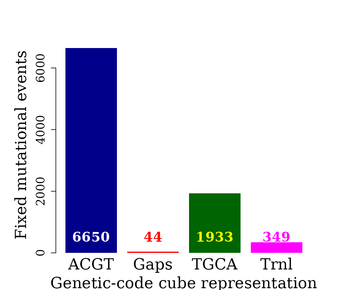
Bar plot automorphism distribution by ranges (regions)
The last result can be summarized by gene regions as follow:
brca1_autm_range <- automorphismByRanges(brca1_autm,
                                  min.len = 2,
                                  num.cores = 10L,
                                  verbose = FALSE)
brca1_autm_range
#> GRangesList object of length 189:
#> $human_1.human_2
#> GRanges object with 3 ranges and 1 metadata column:
#>       seqnames    ranges strand |        cube
#>          <Rle> <IRanges>  <Rle> | <character>
#>   [1]        1     1-349      + |        ACGT
#>   [2]        1       350      + |        Gaps
#>   [3]        1   351-761      + |        ACGT
#>   -------
#>   seqinfo: 1 sequence from an unspecified genome; no seqlengths
#>
#> $human_1.gorilla_1
#> GRanges object with 7 ranges and 1 metadata column:
#>       seqnames    ranges strand |        cube
#>          <Rle> <IRanges>  <Rle> | <character>
#>   [1]        1     1-233      + |        ACGT
#>   [2]        1       234      + |        TGCA
#>   [3]        1   235-349      + |        ACGT
#>   [4]        1       350      + |        Trnl
#>   [5]        1   351-622      + |        ACGT
#>   [6]        1       623      + |        TGCA
#>   [7]        1   624-761      + |        ACGT
#>   -------
#>   seqinfo: 1 sequence from an unspecified genome; no seqlengths
#>
#> $human_1.gorilla_2
#> GRanges object with 7 ranges and 1 metadata column:
#>       seqnames    ranges strand |        cube
#>          <Rle> <IRanges>  <Rle> | <character>
#>   [1]        1     1-233      + |        ACGT
#>   [2]        1       234      + |        TGCA
#>   [3]        1   235-349      + |        ACGT
#>   [4]        1       350      + |        Gaps
#>   [5]        1   351-622      + |        ACGT
#>   [6]        1       623      + |        TGCA
#>   [7]        1   624-761      + |        ACGT
#>   -------
#>   seqinfo: 1 sequence from an unspecified genome; no seqlengths
#>
#> ...
#> <186 more elements>
That is, function automorphismByRanges permits the classification of the pairwise alignment of protein-coding sub-regions based on the mutational events observed on it quantitatively represented as automorphisms on genetic-code cubes.
Searching for automorphisms on permits us a quantitative differentiation between mutational events at different codon positions from a given DNA protein-encoding region. As shown in reference (4)) a set of different cubes can be applied to describe the best evolutionary aminoacid scale highly correlated with aminoacid physicochemical properties describing the observed evolutionary process in a given protein.
More information about this subject can be found in the supporting material from reference (4)) at GitHub GenomeAlgebra_SymmetricGroup, particularly by interacting with the Mathematica notebook Genetic-Code-Scales_of_Amino-Acids.nb.
The automorphism distribution by cubes can be summarized in the bar-plot graphic
cts <- unlist(brca1_autm_range)
counts <- table(cts$cube)

par(family = "serif", cex = 1, font = 2, las = 1)
barplot(counts, main="Automorphism distribution",
        xlab="Genetic-code cube representation",
        col=c("darkblue","red", "darkgreen", "magenta"),
        border = NA, axes = T)
mtext(side = 1,line = -6, at = c(0.7, 1.9, 3.1, 4.3),
      text = paste0( counts ),
      col = c("white", "black", "yellow", "red"))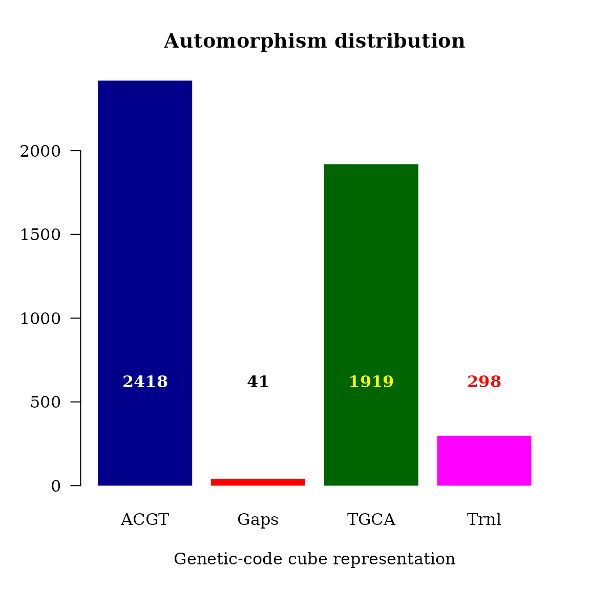
Grouping automorphism by automorphism’s coefficients
Automorphisms with the same automorphism’s coefficients can be grouped.
autby_coef <- automorphism_bycoef(brca1_autm,
                                 verbose = FALSE)
The result is provided with the package
data(autby_coef, package = "GenomAutomorphism")
autby_coef
#> AutomorphismByCoefList object of length 190:
#> $human_1.human_2
#> AutomorphismByCoef object with 239 ranges and 7 metadata columns:
#>         seqnames    ranges strand |        seq1        seq2         aa1         aa2      autm    mut_type        cube
#>            <Rle> <IRanges>  <Rle> | <character> <character> <character> <character> <numeric> <character> <character>
#>     [1]        1     1-238      + |         ATG         ATG           M           M         1         HHH        ACGT
#>     [2]        1     1-238      + |         GAT         GAT           D           D         1         HHH        ACGT
#>     [3]        1     1-238      + |         TTA         TTA           L           L         1         HHH        ACGT
#>     [4]        1     1-238      + |         TCT         TCT           S           S         1         HHH        ACGT
#>     [5]        1     1-238      + |         GCT         GCT           A           A         1         HHH        ACGT
#>     ...      ...       ...    ... .         ...         ...         ...         ...       ...         ...         ...
#>   [235]        1   511-761      + |         CCC         CCC           P           P         1         HHH        ACGT
#>   [236]        1   511-761      + |         CTT         CTT           L           L         1         HHH        ACGT
#>   [237]        1   511-761      + |         CCT         CCT           P           P         1         HHH        ACGT
#>   [238]        1   511-761      + |         ATA         ATA           I           I         1         HHH        ACGT
#>   [239]        1   511-761      + |         TGA         TGA           *           *         1         HHH        ACGT
#>   -------
#>   seqinfo: 1 sequence from an unspecified genome; no seqlengths
#>
#> ...
#> <189 more elements>
As a result of the evolutionary pressure on DNA protein-coding regions (addressed to preserve the aminoacid physicochemical properties and, consequently, the biological functions of the encoded proteins) the highest mutational rate is found in the third base of the codon, followed by the first base, and the lowest rate is found in the second one. DNA bases are classified based on the physicochemical criteria used to ordering the set of codons: number of hydrogen bonds (strong-weak, S-W), chemical type (purine-pyrimidine, Y-R), and chemical groups (amino versus keto, M-K) (see reference 4). Preserved codon positions are labeled with letter “H”. Preserved codon positions are labeled with letter “H” and insertion-mutations identified in the multiple sequence alignment are labeled as “—”.
cts <- unlist(autby_coef)
counts <- table(cts$mut_type[ cts$autm != 1 & cts$autm != -1 ])
counts <- counts[-1] ## remove indel mutations
counts <- sort(counts, decreasing = TRUE)

par(family = "serif", cex.axis = 1.4, font = 2, las = 1,
    cex.main = 1.4, cex.lab = 2)
barplot(counts, main="Automorphism distribution per Mutation type",
        col = colorRampPalette(c("red", "yellow", "blue"))(36),
        border = NA, axes = TRUE,las=2)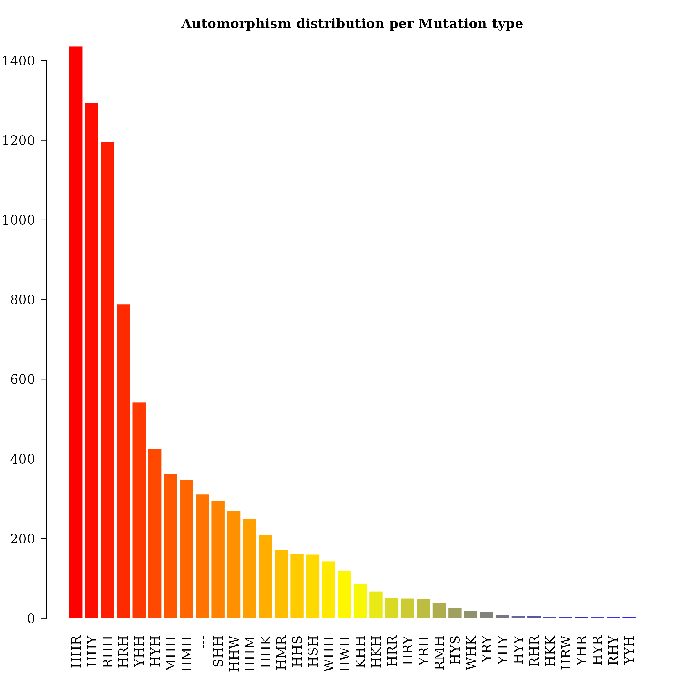
Conserved and non-conserved regions
A specific function is provided to get the coordinates of conserved and non-conserved regions, which can be used in further downstream analyses.
The conserved regions from each pairwise comparison are retrieved typing:
conserv <- conserved_regions(x = brca1_autm)
widths <- width(conserv)
dist <- fitCDF(widths, distNames = c(2, 3, 7, 10, 11, 19, 20), plot = TRUE,
               loss.fun = "cauchy")
#>
#> *** Fitting Log-normal distribution ...
#> .Fitting Done.
#>
#> *** Fitting Half-Normal distribution ...
#> .Fitting Done.
#>
#> *** Fitting Gamma distribution ...
#> .
#>
#> Error in nls.lm(par = PARS, fn = optFun, probfun = funLIST[[i]], quantiles = X,  :
#>   Non-finite (or null) value for a parameter specified!
#> Function model: Gamma
#> Error!
#>
#> *** Fitting Generalized 3P Gamma distribution ...
#> .
#>
#> Error in nls.lm(par = PARS, fn = optFun, probfun = funLIST[[i]], quantiles = X,  :
#>   evaluation of fn function returns non-sensible value!
#> Function model: Generalized 3P Gamma
#> Error!
#>
#> *** Fitting Weibull distribution ...
#> .Fitting Done.
#>
#> *** Fitting Exponential distribution ...
#> .Fitting Done.
#>
#> *** Fitting 2P Exponential distribution ...
#> .Fitting Done.
#>  * Estimating Studentized residuals for Weibull distribution
#>  * Plots for Weibull distribution...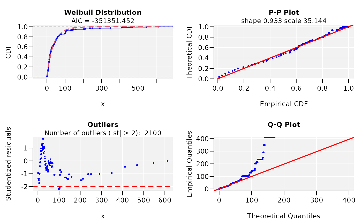
dist
#> weibull CDF model
#> ------
#> Parameters:
#>           Estimate   Std. Error  t value   Pr(>|t|)
#> shape 9.329716e-01 3.777814e-04 2469.607 < 2.22e-16 ***
#> scale 3.514383e+01 1.243175e-02 2826.942 < 2.22e-16 ***
#> ---
#> Signif. codes:  0 '***' 0.001 '**' 0.01 '*' 0.05 '.' 0.1 ' ' 1
#>
#> Residual standard error: 0.0005320935 on 80623 degrees of freedom
#> Number of iterations to termination: 17
#> Reason for termination: Relative error in the sum of squares is at most `ftol'.
#>
#> Goodness of fit:
#>     Adj.R.Square       rho R.Cross.val       AIC
#> gof    0.9999965 0.9999965   0.9957418 -351351.5
par(lwd = 0.5, cex.axis = 2, cex.lab =1.4,
    cex.main = 2, mar=c(5,6,4,4), family = "serif")
hist(widths, 40, freq = FALSE, las = 1, family = "serif",
col = "cyan1", cex.main = 1.2,
main = "Histogram and best fitted CDF model",
xlab = "Conserved region size (bp)", yaxt = "n", ylab="", cex.axis = 1.4)
axis(side = 2, cex.axis = 1.4, las = 2, line = -0.2)
mtext("Density", side = 2, cex = 1.4, line = 4)

x1 <- seq(1, 600, by = 1)
txt <- TeX(r'($\textit{f}(\textit{x}) = \frac{\alpha}{\beta}
    {(\frac{\textit{x}}{\beta})}^{\alpha-1}
    e^{(-\frac{\textit{x}}{\beta})^\alpha}$)')

lines(x1, dweibull(x1,
                  shape = coef(dist$bestfit)[1],
                  scale = coef(dist$bestfit)[2]
                  ),
      col = "red", lwd = 1)
mtext(txt, side = 3, line = -4, cex = 1.8, adj = 0.4)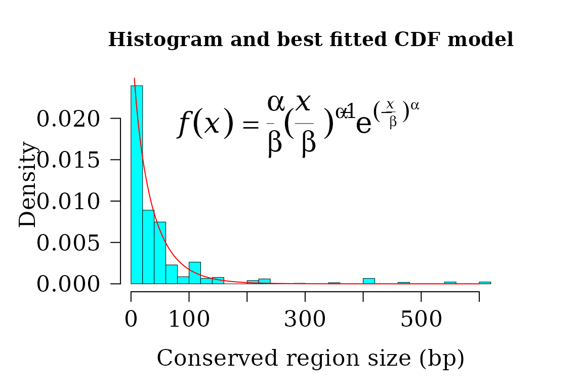
The non-conserved regions from each pairwise comparison are obtained with the same function but different settings:
ncs <- conserved_regions(x = autby_coef, conserved = FALSE)
ncs
#> AutomorphismByCoef object with 8956 ranges and 7 metadata columns:
#>                                    seqnames    ranges strand |        seq1        seq2         aa1         aa2
#>                                       <Rle> <IRanges>  <Rle> | <character> <character> <character> <character>
#>              human_1.gelada_baboon        1         4      + |         TCT         CCT           S           P
#>              human_2.gelada_baboon        1         4      + |         TCT         CCT           S           P
#>            gorilla_1.gelada_baboon        1         4      + |         TCT         CCT           S           P
#>            gorilla_2.gelada_baboon        1         4      + |         TCT         CCT           S           P
#>            gorilla_3.gelada_baboon        1         4      + |         TCT         CCT           S           P
#>                                ...      ...       ...    ... .         ...         ...         ...         ...
#>   silvery_gibbon_1.bolivian_monkey        1       756      + |         CCC         CCT           P           P
#>   silvery_gibbon_3.bolivian_monkey        1       756      + |         CCC         CCT           P           P
#>    golden_monkey_1.bolivian_monkey        1       756      + |         CCC         CCT           P           P
#>    golden_monkey_2.bolivian_monkey        1       756      + |         CCC         CCT           P           P
#>      gelada_baboon.bolivian_monkey        1       756      + |         CCC         CCT           P           P
#>                                         autm    mut_type        cube
#>                                    <numeric> <character> <character>
#>              human_1.gelada_baboon         9         YHH        ACGT
#>              human_2.gelada_baboon         9         YHH        ACGT
#>            gorilla_1.gelada_baboon         9         YHH        ACGT
#>            gorilla_2.gelada_baboon         9         YHH        ACGT
#>            gorilla_3.gelada_baboon         9         YHH        ACGT
#>                                ...       ...         ...         ...
#>   silvery_gibbon_1.bolivian_monkey        59         HHY        ACGT
#>   silvery_gibbon_3.bolivian_monkey        59         HHY        ACGT
#>    golden_monkey_1.bolivian_monkey        59         HHY        ACGT
#>    golden_monkey_2.bolivian_monkey        59         HHY        ACGT
#>      gelada_baboon.bolivian_monkey        59         HHY        ACGT
#>   -------
#>   seqinfo: 1 sequence from an unspecified genome; no seqlengths
Subsetting regions of interest
The application of some of the available bioinformatic tools is straightforward. For example, knowing the positions for the conserved and non-conserved regions, we can subset into the alignment region of potential interest.
The coordinates carrying mutational events are:
sort(unique(start(ncs)))
#>   [1]   4   6   7  11  15  20  25  29  45  52  60  63  71  74  77  85  86  91  94 100 101 104 113 122 124 128 132 138
#>  [29] 139 142 143 146 148 151 152 155 159 161 164 167 170 172 175 176 181 182 190 191 193 194 196 205 214 216 225 227
#>  [57] 231 233 234 239 240 241 244 245 247 251 252 253 254 267 269 270 275 276 279 281 282 286 287 292 293 299 300 301
#>  [85] 310 318 319 323 324 326 328 329 330 331 333 339 340 350 357 359 360 361 363 369 370 374 375 376 378 394 396 399
#> [113] 402 406 407 410 417 418 421 425 428 431 433 435 438 442 443 444 445 447 453 458 461 466 472 476 477 478 480 482
#> [141] 483 485 486 487 489 499 501 502 503 505 507 509 510 511 516 518 521 522 523 525 526 532 535 536 537 545 549 550
#> [169] 552 554 560 564 568 569 572 576 578 584 585 590 597 601 602 605 623 647 653 654 659 660 665 669 678 681 683 685
#> [197] 693 701 702 703 704 716 726 728 730 731 748 749 753 756
We will use function DNAStringSet from the Bioconductor R package Biostrings to subset the MSA of primate cytochrome c.
brca1_aln_region <- DNAStringSet(brca1_aln, start = 37*3 - 2, end = 42*3)
brca1_aln_region
#> DNAStringSet object of length 20:
#>      width seq                                                                                      names
#>  [1]    18 ACAAAGTGTGACCACATA                                                                       NM_007298.3:20-22...
#>  [2]    18 ACAAAGTGTGACCACATA                                                                       U64805.1:1-2280_H...
#>  [3]    18 ACAAAGTGTGACCACATA                                                                       XM_031011560.1:23...
#>  [4]    18 ACAAAGTGTGACCACATA                                                                       XM_031011561.1:23...
#>  [5]    18 ACAAAGTGTGACCACATA                                                                       XM_031011562.1:16...
#>  ...   ... ...
#> [16]    18 ACAAAGTGTGACCACATA                                                                       XM_032163758.1:13...
#> [17]    18 ACAAAGTGTGACCACATA                                                                       XM_030923119.1:18...
#> [18]    18 ACAAAGTGTGACCACATA                                                                       XM_030923118.1:18...
#> [19]    18 ACAAAGTGTGACCACATA                                                                       XM_025363316.1:14...
#> [20]    18 ACAAAGTGTGACCACATA                                                                       XM_039475995.1:49...
Next, function ggseqlogo from the R package ggseqlogo will be applied to get the logo sequence from the selected MSA region.
ggseqlogo( as.character(brca1_aln_region) )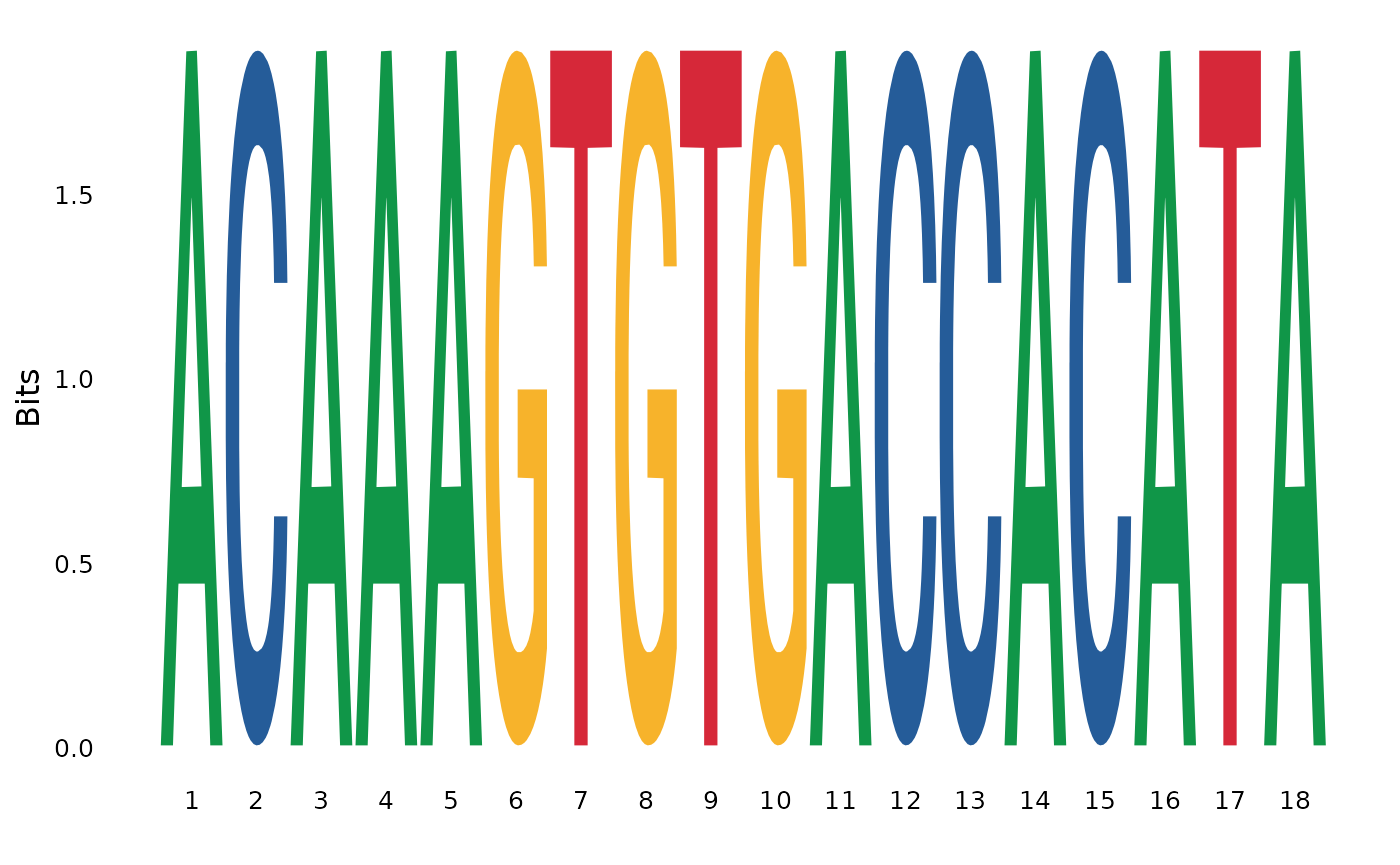
The corresponding aminoacid sequence will be
brca1_aln_region_aa = translate(brca1_aln_region)
brca1_aln_region_aa
#> AAStringSet object of length 20:
#>      width seq                                                                                      names
#>  [1]     6 TKCDHI                                                                                   NM_007298.3:20-22...
#>  [2]     6 TKCDHI                                                                                   U64805.1:1-2280_H...
#>  [3]     6 TKCDHI                                                                                   XM_031011560.1:23...
#>  [4]     6 TKCDHI                                                                                   XM_031011561.1:23...
#>  [5]     6 TKCDHI                                                                                   XM_031011562.1:16...
#>  ...   ... ...
#> [16]     6 TKCDHI                                                                                   XM_032163758.1:13...
#> [17]     6 TKCDHI                                                                                   XM_030923119.1:18...
#> [18]     6 TKCDHI                                                                                   XM_030923118.1:18...
#> [19]     6 TKCDHI                                                                                   XM_025363316.1:14...
#> [20]     6 TKCDHI                                                                                   XM_039475995.1:49...
And the corresponding aminoacid sequence logo will is
ggseqlogo( as.character(brca1_aln_region_aa) )![]()
That is, the first mutational event reported in the codon sequence correspond to a synonymous mutation.
References
1. Sanchez R, Morgado E, Grau R. Gene algebra from a genetic code algebraic structure. J Math Biol. 2005 Oct;51(4):431-57. doi: 10.1007/s00285-005-0332-8. Epub 2005 Jul 13. PMID: 16012800. ( PDF).
2. Robersy Sanchez, Jesús Barreto (2021) Genomic Abelian Finite Groups. doi: 10.1101/2021.06.01.446543.
3. M. V José, E.R. Morgado, R. Sánchez, T. Govezensky, The 24 possible algebraic representations of the standard genetic code in six or in three dimensions, Adv. Stud. Biol. 4 (2012) 119–152.PDF.
4. R. Sanchez. Symmetric Group of the Genetic–Code Cubes. Effect of the Genetic–Code Architecture on the Evolutionary Process MATCH Commun. Math. Comput. Chem. 79 (2018) 527-560. PDF.