P-P plot of Two-dimensional Copulas

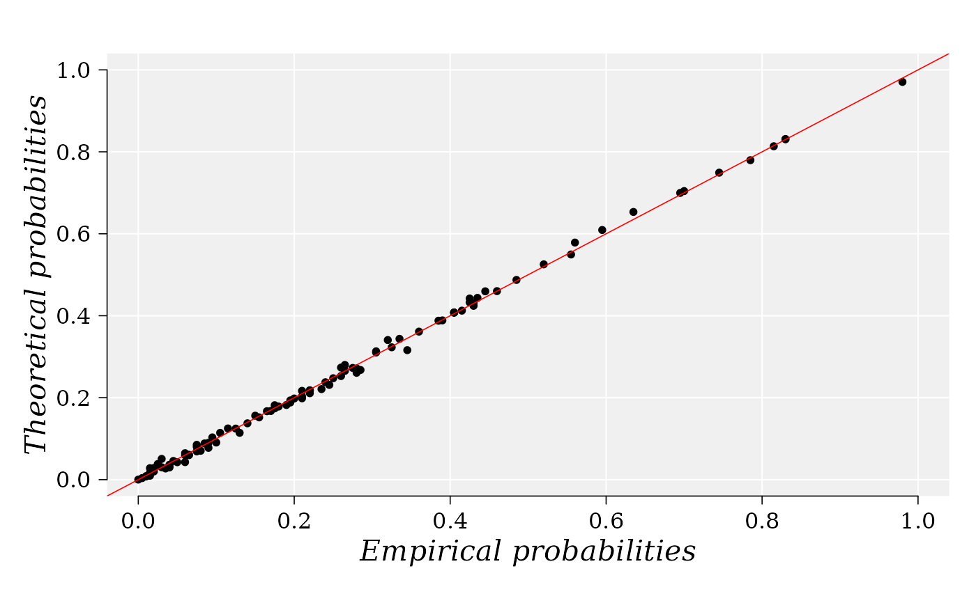
The function build the P-P plot of Two-dimensional Copulas upon the knowledge of the margin distribution provided by the user. The empirical probabilities are computed using function empCopula from package [copula-package]{copula}.

ppCplot(
  X,
  Y,
  copula = NULL,
  margins = NULL,
  paramMargins = NULL,
  npoints = 100,
  method = "ml",
  smoothing = c("none", "beta", "checkerboard"),
  ties.method = "max",
  xlab = "Empirical probabilities",
  ylab = "Theoretical probabilities",
  glwd = 1.2,
  bgcol = "grey94",
  gcol = "white",
  dcol = "red",
  dlwd = 0.8,
  tck = NA,
  tcl = -0.3,
  xlwd = 0.8,
  ylwd = 0.8,
  xcol = "black",
  ycol = "black",
  cex.xtitle = 1.3,
  cex.ytitle = 1.3,
  padj = -1,
  hadj = 0.7,
  xcex = 1.3,
  ycex = 1.3,
  xline = 1.6,
  yline = 2.1,
  xfont = 3,
  yfont = 3,
  family = "serif",
  lty = 1,
  bty = "n",
  col = "black",
  xlim = c(0, 1),
  ylim = c(0, 1),
  pch = 20,
  las = 1,
  mar = c(4, 4, 2, 1),
  font = 3,
  cex = 1,
  seed = 132,
  ...
)

Arguments

X: Numerical vector with the observations from the first margin distribution.
Y: Numerical vector with the observations from the second margin distribution.
copula: A copula object from class Mvdc or string specifying all the name for a copula from package copula-package.
margins: A character vector specifying all the parametric marginal distributions. See details below.
paramMargins: A list whose each component is a list (or numeric vectors) of named components, giving the parameter values of the marginal distributions. See details below.
npoints: Number of points used to build the P-P plot. The
method: A character string specifying the estimation method to be used to estimate the dependence parameter(s) (if the copula needs to be estimated) see fitCopula.
smoothing: character string specifying whether the empirical distribution function (for F.n()) or copula (for C.n()) is computed (if smoothing = "none"), or whether the empirical beta copula (smoothing = "beta") or the empirical checkerboard copula (smoothing = "checkerboard") is computed (see empCopula.
ties.method: character string specifying how ranks should be computed if there are ties in any of the coordinate samples of x; passed to pobs (see empCopula.
xlab: A label for the x axis, defaults to a description of x.
ylab: A label for the y axis, defaults to a description of y.
glwd: Grid line width.
bgcol: Grid background color.
gcol: Grid line color
dcol: Diagonal line color.
dlwd: Diagonal line color.
tck: The length of tick marks as a fraction of the smaller of the width or height of the plotting region. If tck >= 0.5 it is interpreted as a fraction of the relevant side, so if tck = 1 grid lines are drawn. The default setting (tck = NA) is to use tcl = -0.5.
tcl: The length of tick marks as a fraction of the height of a line of text. The default value is -0.5; setting tcl = NA sets tck = -0.01 which is S' default.
xlwd: X-axis line width.
ylwd: Y-axis line width.
xcol: X-axis line color.
ycol: Y-axis line color.
cex.xtitle: Cex for x-axis title.
cex.ytitle: Cex for y-axis title.
padj: adjustment for each tick label perpendicular to the reading direction. For labels parallel to the axes, padj = 0 means right or top alignment, and padj = 1 means left or bottom alignment. This can be a vector given a value for each string, and will be recycled as necessary.
hadj: adjustment (see par("adj")) for all labels parallel (‘horizontal’) to the reading direction. If this is not a finite value, the default is used (centring for strings parallel to the axis, justification of the end nearest the axis otherwise).
xcex, ycex: A numerical value giving the amount by which axis labels should be magnified relative to the default.
xline, yline: On which margin line of the plot the x & y labels must be placed, starting at 0 counting outwards (see mtext).
xfont, yfont: An integer which specifies which font to use for x & y axes titles (see par).
family, lty, bty, col, xlim, ylim, pch, las, mar, font: Graphical parameters (see par).
cex: A numerical value giving the amount by which plotting text and symbols should be magnified relative to the default. This starts as 1 when a device is opened, and is reset when the layout is changed, e.g. by setting mfrow.
seed: An integer used to set a 'seed' for random number generation.
...: Other graphical parameters to pass to functions: abline, mtext and axis.

Value

The P-P plot and invisible temporary object with the information to build the graphic which can be assigned to a variable to use in further plots or analyses.

Details

Empirical and theoretical probabilities are estimated using the quantiles generated with the margin quantile functions. Nonlinear fit of margin distributions can be previously accomplished using any of the functions fitCDF, fitdistr, or function fitMixDist for the case where the margins are mixture of distributions. npoints random uniform and iid numbers from the interval [0, 1] are generated and used to evaluate the quantile margin distribution functions. Next, the quantiles are used to compute the empirical and theoretical copulas, which will be used to estimate the corresponding probabilities.

Author

Robersy Sanchez (https://genomaths.com).

Examples

set.seed(12)
margins <- c("lnorm", "norm")
## Random variates from normal distributions
X <- rlnorm(200, meanlog = -0.5, sdlog = 3.1)
Y <- rnorm(200, mean = 0, sd = 6)
cor(X, Y) ## Correlation between X and Y
#> [1] -0.0126086

parMargins <- list(
    list(meanlog = 0.5, sdlog = 3.1),
    list(mean = 0, sd = 10)
)

copula <- "normalCopula"

## The information to build the graphic is stored in object 'g'.
g <- ppCplot(
    X = X, Y = Y, copula = "normalCopula", margins = margins,
    paramMargins = parMargins, npoints = 100
)