Probability density function (PDF), cummulative density function (CDF), quantile function and random generation for the Half-normal (hnorm) distribution.
dhnorm(x, theta = 1, mu = 0, log = FALSE)

phnorm(q, theta = 1, mu = 0, lower.tail = TRUE, log.p = FALSE)

qhnorm(p, theta = 1, mu = 0, sigma = NULL, lower.tail = TRUE, log.p = FALSE)

rhnorm(n, theta = 1, mu = 0)

theta2sigma(theta)

sigma2theta(sigma)
Arguments
- x, q
numeric vector, \(x > \mu\) and \(q > \mu\)
- theta
numerical parameter, strictly positive (default 1).
- mu
location parameter (\(\mu\)).
- lower.tail
logical; if TRUE (default), probabilities are P[X<=x], otherwise, P[X > x]
- log.p
logical; if TRUE, probabilities/densities p are returned as log(p).
- sigma
Standard deviation of the normal distribution. Here, \(\sigma = \sqrt \pi/(\theta\sqrt 2)\)
- n
number of observations
Value
Half-normal PDF values (theta parameter) for dhnorm, Half-normal probability for phnorm, quantiles or Half-normal random generated values for rhnorm.
Details
An alternative parameterization to avoid issues when sigma is near zero is applied by using a scaled precision (inverse of the variance) obtained by setting \(\theta = \sqrt(\pi)/(\sigma*\sqrt(2))\). Details about these functions can be found in Wikipedia and in MathWorld and MathWorks to see the distribution with location parameter \(\mu\). Notice that \(\theta = 1\) means \(\sigma = \sqrt \pi/\sqrt 2\).
Examples
set.seed(123) # set a seed
sigma <- 1.2
theta <- sigma2theta(sigma)
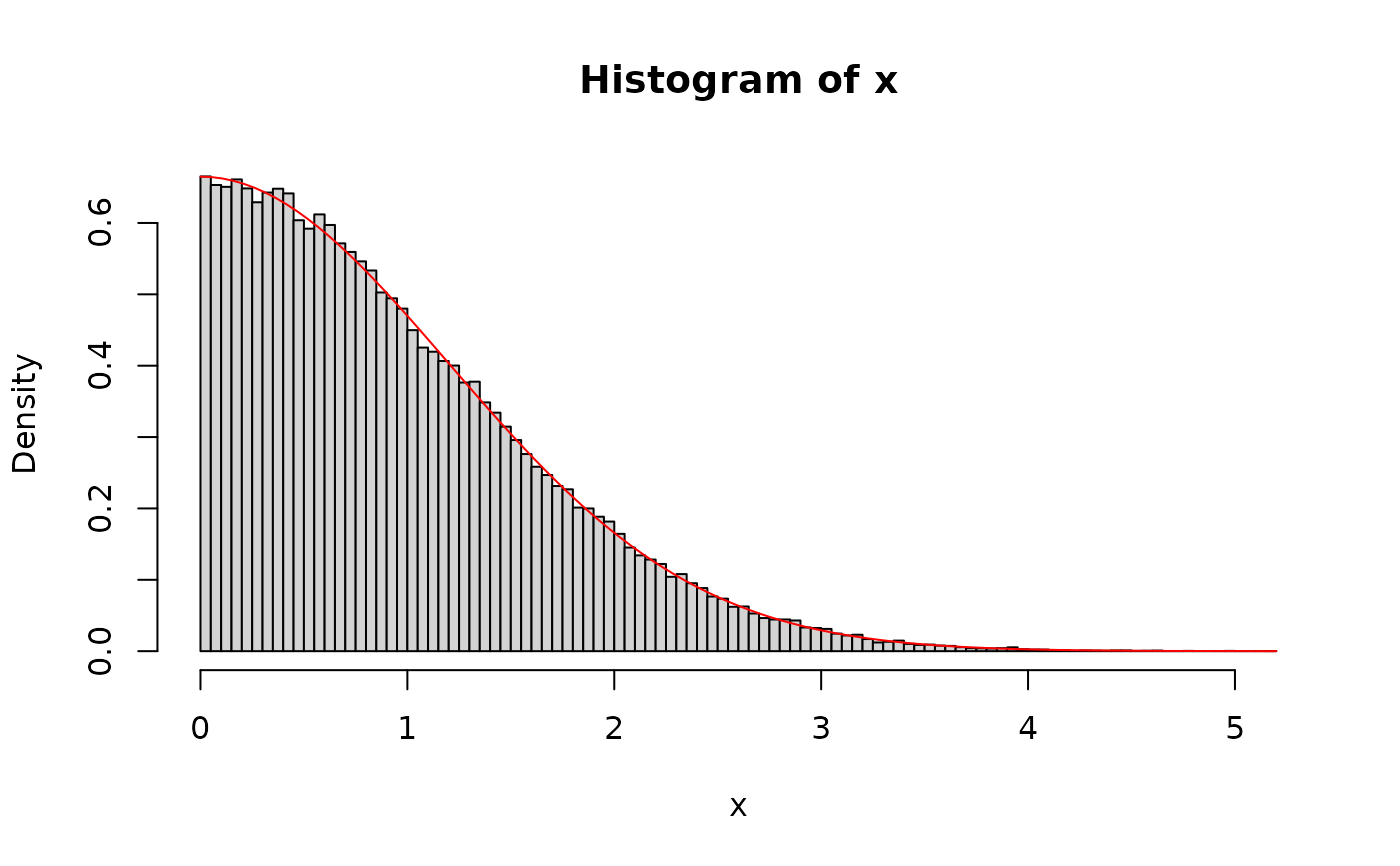
x <- rhnorm(n = 1e5, theta = theta)
hist(x, 100, freq = FALSE)
curve(dhnorm(x, theta = theta), col = "red", add = TRUE)


#' # Checking the function outputs for the logarithms of probabilities
x <- rhnorm(n = 10, theta = sigma2theta(2))
x1 <- phnorm(x, theta = sigma2theta(2), log = TRUE)
x2 <- phnorm(x, theta = sigma2theta(2), log = FALSE)
all(round(x1, 8) == round(log(x2), 8))
#> [1] TRUE

x3 <- dhnorm(x, theta = sigma2theta(2), log = TRUE)
x4 <- dhnorm(x, theta = sigma2theta(2), log = FALSE)
all(round(x3, 8) == round(log(x4), 8))
#> [1] TRUE